Lecture 7 Structure from Motion (SfM)
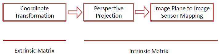
Camera Calibration 相机标定
The process of camera calibration is the process from world coordinates to image sensor, we focus on the four coordinates:
- World Coordinates (世界坐标系)
- Camera Coordinates (相机坐标系)
- Image Plane (图像坐标系)
- Image Sensor (像素坐标系)
The parameters in the first two transform matrices are called Camera Extrinsics (相机外参); the parameters in the last two transform matrices are called Camera Intrinsics (相机内参).
Principle Analysis
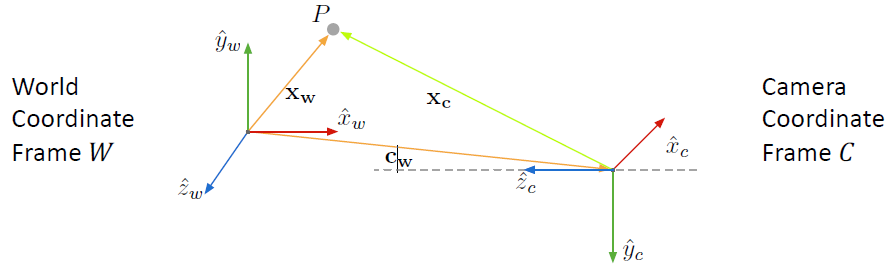
Coordinate transformation is from world coordinates to camera coordinates.
Feature
This transformation is Rigid Body Transformation 刚体变换 (only rotation and translation), corresponding to a rotation matrix \(R\) (which is also orthonormal (单位正交)) and translation vector \(c_w\).
\[
\mathbf{x}_c = R(\mathbf{x}_w - \mathbf{c}_w) = R \mathbf{x}_w - R \mathbf{c}_w \overset{\Delta}{=\!=} R \mathbf{x}_w + \mathbf{t},\ \ \text{ where } \mathbf{t } = -R \mathbf{c}_w.
\]
Thus this transformation can be represented by \(R\) and \(\mathbf{t}\) to indicate equivalently.
\[
\mathbf{x}_c = \begin{bmatrix} x_c \\ y_c \\ z_c \end{bmatrix}
=
\begin{bmatrix}
r_{11} & r_{12} & r_{13} \\
r_{21} & r_{22} & r_{23} \\
r_{31} & r_{32} & r_{33} \\
\end{bmatrix}
\begin{bmatrix}
x_w \\ y_w \\ z_w
\end{bmatrix}
+
\begin{bmatrix}
t_x \\ t_y \\ t_z
\end{bmatrix}.
\]
We also consider the homogenous coordinates,
\[
\mathbf{\tilde x}_c = \begin{bmatrix} x_c \\ y_c \\ z_c \\ 1\end{bmatrix}
=
\begin{bmatrix}
r_{11} & r_{12} & r_{13} & t_x \\
r_{21} & r_{22} & r_{23} & t_y\\
r_{31} & r_{32} & r_{33} & t_z\\
0 & 0 & 0 & 1
\end{bmatrix}
\begin{bmatrix}
x_w \\ y_w \\ z_w \\ 1
\end{bmatrix}.
\]
Extrinsic Matrix 外参矩阵
\[
M_{ext} =
\begin{bmatrix}
R_{3\times 3} & \mathbf{t} \\
\mathbf{0}_{1\times 3} & 1
\end{bmatrix}
=
\begin{bmatrix}
r_{11} & r_{12} & r_{13} & t_x \\
r_{21} & r_{22} & r_{23} & t_y\\
r_{31} & r_{32} & r_{33} & t_z\\
0 & 0 & 0 & 1
\end{bmatrix},
\]
or omitting the last row,
\[
M_{ext} =
\begin{bmatrix}
R_{3\times 3} & \mathbf{t} \\
\end{bmatrix}
=
\begin{bmatrix}
r_{11} & r_{12} & r_{13} & t_x \\
r_{21} & r_{22} & r_{23} & t_y\\
r_{31} & r_{32} & r_{33} & t_z\\
\end{bmatrix}.
\]
Perspective Projection
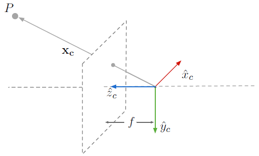
Perspective projection is from camera coordinates to image plane.
We have discuss this part in the previous Lectures, thus we skip it and just leave the conclusion.
\[
\begin{bmatrix}
x_i \\ y_i \\ 1
\end{bmatrix}
\cong
\begin{bmatrix}
f & 0 & 0 & 0 \\
0 & f & 0 & 0 \\
0 & 0 & 1 & 0
\end{bmatrix}
\begin{bmatrix}
x_c \\
y_c \\
z_c \\
1
\end{bmatrix}
\]
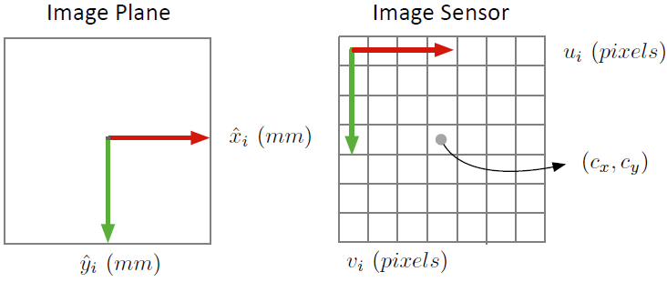
Image Plane to Image Sensor Mapping
pixel (像素点)
Note that since the production and demand, each pixel is not necessarily a square, but a rectangle instead. Compare to the origin image, it has a certain degree of scaling. This discussion also appears in video making.
In addition, since the origin of image plane is at the center of the image, while the origin of image sensor is at the top left corner, we need some tranlation for the coordinate transformation.
\[
\begin{aligned}
u &= m_x f \frac{x_c}{z_c} + c_x, \\
v &= m_y f \frac{y_c}{z_c} + c_y.
\end{aligned}
\]
Combining two transformations above, and denoting \(f_x = m_x f\), \(f_y = m_y f\),
then the transformation from camera coordinates to image sensor is
\[
\mathbf{\tilde{u}}
=
\begin{bmatrix}
u \\ v \\ w
\end{bmatrix}
\cong
\begin{bmatrix}
f_x & 0 & c_x & 0 \\
0 & f_y & c_y & 0 \\
0 & 0 & 1 & 0
\end{bmatrix}
\begin{bmatrix}
x_c \\
y_c \\
z_c \\
1
\end{bmatrix}.
\]
Intrinsic Matrix 内参矩阵
\[
M_{int} =
\begin{bmatrix}
f_x & 0 & c_x & 0 \\
0 & f_y & c_y & 0 \\
0 & 0 & 1 & 0
\end{bmatrix},
\]
or
\[
K =
\begin{bmatrix}
f_x & 0 & c_x \\
0 & f_y & c_y \\
0 & 0 & 1
\end{bmatrix}.
\]
Projection Matrix \(P\)
World to Camera
\[
\begin{bmatrix} x_c \\ y_c \\ z_c \\ 1\end{bmatrix}
=
\begin{bmatrix}
r_{11} & r_{12} & r_{13} & t_x \\
r_{21} & r_{22} & r_{23} & t_y\\
r_{31} & r_{32} & r_{33} & t_z\\
0 & 0 & 0 & 1
\end{bmatrix}
\begin{bmatrix}
x_w \\ y_w \\ z_w \\ 1
\end{bmatrix},
\]
\[
\mathbf{\tilde u} = M_{int}\mathbf{\tilde x}_c.
\]
Camera to Pixel
\[
\begin{bmatrix}
u \\ v \\ w
\end{bmatrix}
\cong
\begin{bmatrix}
f_x & 0 & c_x & 0 \\
0 & f_y & c_y & 0 \\
0 & 0 & 1 & 0
\end{bmatrix}
\begin{bmatrix}
x_c \\
y_c \\
z_c \\
1
\end{bmatrix},
\]
\[
\mathbf{\tilde x}_c = M_{ext}\mathbf{\tilde x}_w.
\]
Thus
\[
\mathbf{\tilde u} = M_{int}M_{ext} \mathbf{\tilde x}_w = P \mathbf{\tilde x},
\]
where \(P\) is called Projection Matrix.
\[
\begin{bmatrix}
u \\ v \\ w
\end{bmatrix}
\cong
\begin{bmatrix}
p_{11} & p_{12} & p_{13} & p_{14} \\
p_{21} & p_{22} & p_{23} & p_{24} \\
p_{31} & p_{32} & p_{33} & p_{34} \\
p_{41} & p_{42} & p_{43} & p_{44}
\end{bmatrix}
\begin{bmatrix}
x_w \\
y_w \\
z_w \\
1
\end{bmatrix}.
\]
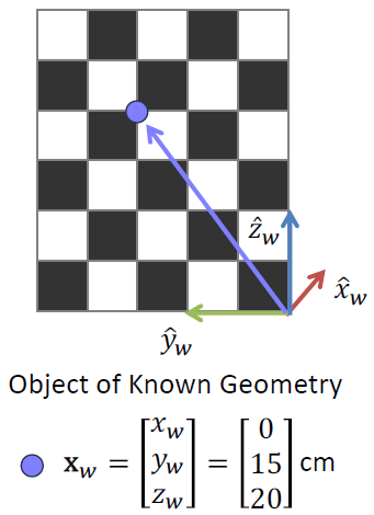
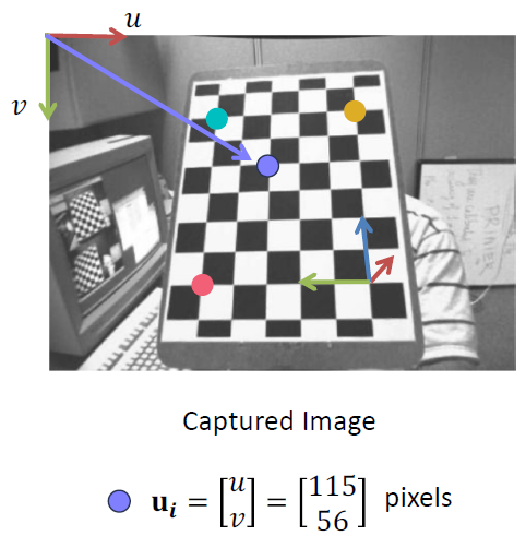
Step 1. Capture an image of an object with known geometry.
Step 2. Identify correspondences (Image Matching 图像匹配) between 3D scene points and image points.
Step 3. For each corresponding point \(i\), we get
\[
\begin{bmatrix}
u^{(i)} \\ v^{(i)} \\ w^{(i)}
\end{bmatrix}
\cong
\begin{bmatrix}
p_{11} & p_{12} & p_{13} & p_{14} \\
p_{21} & p_{22} & p_{23} & p_{24} \\
p_{31} & p_{32} & p_{33} & p_{34} \\
p_{41} & p_{42} & p_{43} & p_{44}
\end{bmatrix}
\begin{bmatrix}
x_w^{(i)} \\
y_w^{(i)} \\
z_w^{(i)} \\
1
\end{bmatrix}.
\]
\[
\begin{aligned}
u^{(i)} &= \frac{p_{11}x_w^{(i)} + p_{12}y_w^{(i)} + p_{13}z_w^{(i)} + p_{14}}{p_{31}x_w^{(i)} + p_{32}y_w^{(i)} + p_{33}z_w^{(i)} + p_{34}}, \\
v^{(i)} &= \frac{p_{21}x_w^{(i)} + p_{22}y_w^{(i)} + p_{23}z_w^{(i)} + p_{24}}{p_{31}x_w^{(i)} + p_{32}y_w^{(i)} + p_{33}z_w^{(i)} + p_{34}}
\end{aligned}.
\]
Step 4. Rearrange.
\[
\small
\begin{bmatrix}
x_w^{(1)} & y_w^{(1)} & z_w^{(1)} & 1 & 0 & 0 & 0 & 0 & -u_1x_w^{(1)} & -u_1y_w^{(1)} & -u_1z_w^{(1)} & -u_1 \\
0 & 0 & 0 & 0 & x_w^{(1)} & y_w^{(1)} & z_w^{(1)} & 1 & -v_1x_w^{(1)} & -v_1y_w^{(1)} & -v_1z_w^{(1)} & -v_1 \\
\vdots & \vdots & \vdots & \vdots & \vdots & \vdots & \vdots & \vdots & \vdots & \vdots & \vdots & \vdots \\
x_w^{(i)} & y_w^{(i)} & z_w^{(i)} & 1 & 0 & 0 & 0 & 0 & -u_ix_w^{(i)} & -u_iy_w^{(i)} & -u_iz_w^{(i)} & -u_i \\
0 & 0 & 0 & 0 & x_w^{(i)} & y_w^{(i)} & z_w^{(i)} & 1 & -v_ix_w^{(i)} & -v_iy_w^{(i)} & -v_iz_w^{(i)} & -v_i \\
\vdots & \vdots & \vdots & \vdots & \vdots & \vdots & \vdots & \vdots & \vdots & \vdots & \vdots & \vdots \\
x_w^{(n)} & y_w^{(n)} & z_w^{(n)} & 1 & 0 & 0 & 0 & 0 & -u_nx_w^{(n)} & -u_ny_w^{(n)} & -u_nz_w^{(n)} & -u_n \\
0 & 0 & 0 & 0 & x_w^{(n)} & y_w^{(n)} & z_w^{(n)} & 1 & -v_nx_w^{(n)} & -v_ny_w^{(n)} & -v_nz_w^{(n)} & -v_n \\
\end{bmatrix}
\begin{bmatrix}
p_{11} \\ p_{12} \\ p_{13} \\ p_{14} \\
p_{21} \\ p_{22} \\ p_{23} \\ p_{24} \\
p_{31} \\ p_{32} \\ p_{33} \\ p_{34}
\end{bmatrix}
=
\begin{bmatrix}
0 \\ 0 \\ 0 \\ 0 \\
0 \\ 0 \\ 0 \\ 0 \\
0 \\ 0 \\ 0 \\ 0
\end{bmatrix},
\]
\[
i.e.\ \ A \mathbf{p} = 0.
\]
Step 5. Solve for \(P\).
Similarly, we can give some constraints.
- Option 1. \(p_{34} = 1\).
- Option 2. \(||p|| = 1\).
Thus the degree of freedom is \(11\),at least \(6\) pairs of points.
Similarly we need to minimize \(||\mathbf{Ap - 0}|| = \mathbf{||Ap||}\).
And also, if we select the constraint that the vector norm is \(1\), then we only need to determine the direction of \(\mathbf{p}\), denoted by \(\mathbf{\hat p}\), and \(\mathbf{\hat p}\) is the corresponding eigenvector of the eigenvalue of \(\mathbf{A^{T}A}\).
Step 6. From \(P\) to Answers
\[
\begin{bmatrix}
p_{11} \\ p_{12} \\ p_{13} \\ p_{14} \\
p_{21} \\ p_{22} \\ p_{23} \\ p_{24} \\
p_{31} \\ p_{32} \\ p_{33} \\ p_{34}
\end{bmatrix}
=
\begin{bmatrix}
f_x & 0 & c_x & 0 \\
0 & f_y & c_y & 0 \\
0 & 0 & 1 & 0
\end{bmatrix}
\begin{bmatrix}
r_{11} & r_{12} & r_{13} & t_x \\
r_{21} & r_{22} & r_{23} & t_y\\
r_{31} & r_{32} & r_{33} & t_z\\
0 & 0 & 0 & 1
\end{bmatrix}.
\]
Notice that
\[
\begin{bmatrix}
p_{11} \\ p_{12} \\ p_{13} \\
p_{21} \\ p_{22} \\ p_{23} \\
p_{31} \\ p_{32} \\ p_{33}
\end{bmatrix}
=
\begin{bmatrix}
f_x & 0 & c_x \\
0 & f_y & c_y \\
0 & 0 & 1
\end{bmatrix}
\begin{bmatrix}
r_{11} & r_{12} & r_{13} \\
r_{21} & r_{22} & r_{23} \\
r_{31} & r_{32} & r_{33} \\
\end{bmatrix}
= KR.
\]
where \(K\) is an Upper Right Triangular Matrix, \(R\) is an Orthonormal Matrix).
From QR Factorization, we know that the solution of \(K\) and \(R\) is unique.
And
\[
\begin{bmatrix}
p_{14} \\ p_{24} \\ p_{34}
\end{bmatrix}
=
\begin{bmatrix}
f_x & 0 & c_x \\
0 & f_y & c_y \\
0 & 0 & 1
\end{bmatrix}
\begin{bmatrix}
t_x \\ t_y \\ t_z
\end{bmatrix}
= K \mathbf{t}.
\]
Thus we can solve
\[
\mathbf{t} = K^{-1}
\begin{bmatrix}
p_{14} \\ p_{24} \\ p_{34}
\end{bmatrix}.
\]
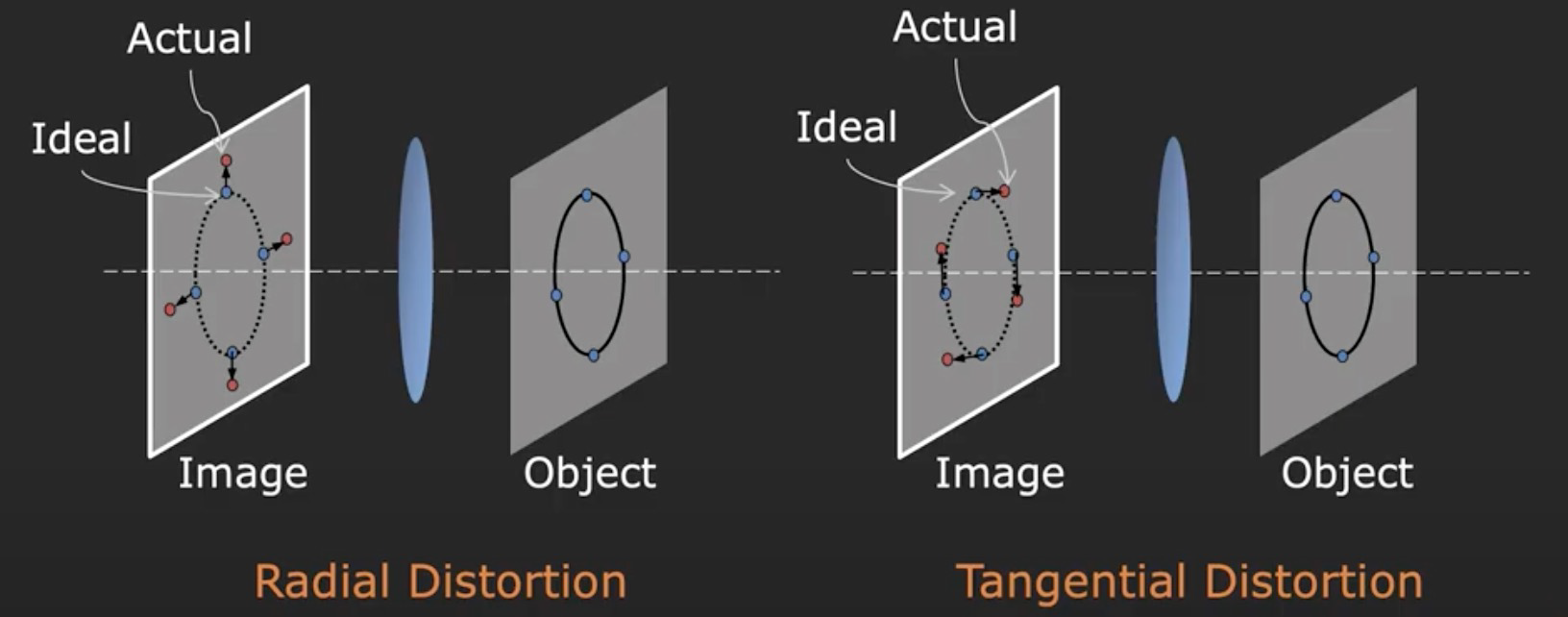
Problem: Distortion
In fact, camera itself has some coefficients of distortion, we ignore its effects here.
Perspective-n-Point Problem (PnP 问题)
Weakning the premises, suppose camera intrinsics are known (namely matrix \(K\)), we need to solve camera extrinsics (namely matrix \(R\) and \(\mathbf{t}\)), namely camera pose (相机姿态).
We have some methods to solve this problem.
It's the method mentioned above. First solve out \(P\), and from \(K\) solve out \(R\) and \(\mathbf{t}\).
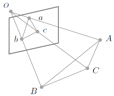
P3P
The question is with the coordinates \(a, b, c, A, B, C\) known, find out the coordinate of \(O\).
- First, we need at least \(3\) pairs of points.
Intermediates.
- From Cosine Theorem,
\[
\begin{aligned}
OA^2 + OB^2 - 2 OA \cdot OB \cos \angle AOB &= AB^2, \\
OA^2 + OC^2 - 2 OB \cdot OC \cos \angle BOC &= BC^2, \\
OA^2 + OC^2 - 2 OA \cdot OC \cos \angle AOC &= AC^2.
\end{aligned}
\]
- Let \(x = \dfrac{OA}{OC}\), \(y = \dfrac{OB}{OC}\), \(v = \dfrac{AB^2}{OC^2}\), \(u = \dfrac{BC^2}{AB^2}\), \(w = \dfrac{AC^2}{AB^2}\), and simplify the equations above. We have
\[
\begin{aligned}
(1 - u)y^2 - ux^2 - cos \angle BOC y + 2uxy \cos \angle AOB + 1 &= 0, \\
(1 - w)x^2 - wy^2 - cos \angle AOC y + 2wxy \cos \angle AOB + 1 &= 0.
\end{aligned}
\]
- The equations above are Binary Quadratic Equation (二元二次方程组) with FOUR solutions, where two of them are the cases that the coordinate of \(O\) is between \(\text{Plane} ABC\) and \(\text{Plane} abc\), thus discarded.
- We need one ore pair of points for the unique solution, thus we need \(4\) pairs of points in total.
PnP
The idea of PnP is to minimize Reprojection Error (重投影误差).
\[
\mathop{\arg\min\limits_{R, \mathbf{t}}} \sum\limits_i ||(p_i, K(RP_i + \mathbf{t})||^2,
\]
where, \(p_i\) is the 2D coordinates of the projection plane and \(P_i\) is the 3D coordinates in space.
The method is FIRST initializing by P3P,and SECOND optimizing by Gauss-Newton method.
EPnP
- one of the most popluar methods.
- time complexity \(O(N)\).
- high accuracy.
The general method is to solve by the linear combinations of four pairs of control points.
Two-frame Structure from Motion
Stereo vision 立体视觉
Compute 3D structure of the scene and camera poses from views (images).
Two-frame SfM is aimed at solving a problem: Given two images and the intrinsic matrices (\(K_l(3 \times 3)\) and \(K_r(3 \times 3)\)),find camera pose and the coordinates of the captured objects.
Principle Induction 原理推导
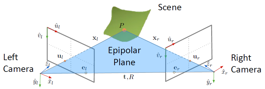
Epipolar Geometry 对极几何
Epipolar geometry describes a geometry relation of \(u_l\), \(u_r\), which are the 2D projections of a 3D point \(P\) in two views. And through this relation build up the transformation of the two cameras (namely find \(R\) and \(\mathbf{t}\)).
Definition
- Epipole 对极点: the projection of one camera in the other camera, i.e. \(e_l\) and \(e_r\) in the picture above.
- For given two camera, \(e_l\) and \(e_r\) are unique.
- Epipolar Plane of Scene Point P 关于 P 点的对极面: the plane formed by Scene Point \(P\), \(O_l\) and \(O_r\).
- Each scene point has a unique corresponding epipolar plane.
- Epipoles are on the epipolar plane.
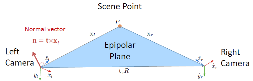
Essential Matrix \(E\) 基本矩阵
For an epipolar plane, we have
\[
\begin{aligned}
\mathbf{n} = \mathbf{t} \times \mathbf{x}_l, \\
\mathbf{x}_l \cdot (\mathbf{t} \times \mathbf{x}_l) = 0.
\end{aligned}
\]
where \(\mathbf{n}\) is called Normal Vector.
Suppose the right camera transforms with a rigid body transformation to the left camera, namely
\[
\begin{aligned}
\mathbf{x}_l &= R \mathbf{x}_r + \mathbf{t}, \\
\begin{bmatrix}
x_l \\ y_l \\ z_l
\end{bmatrix}
&=
\begin{bmatrix}
r_{11} & r_{12} & r_{13} \\
r_{21} & r_{22} & r_{23} \\
r_{31} & r_{32} & r_{33}
\end{bmatrix}
\begin{bmatrix}
x_r \\ y_r \\ y_r
\end{bmatrix}
+
\begin{bmatrix}
t_x \\ t_y \\ t_z
\end{bmatrix}.
\end{aligned}
\]
Moreover, we have
\[
\begin{aligned}
\begin{bmatrix}
x_l & y_l & z_l
\end{bmatrix}
\begin{bmatrix}
t_yz_l - t_zy_l \\
t_zx_l - t_xz_l \\
t_xy_l - t_yx_l
\end{bmatrix}
= 0,
& \text{ Cross-product definition} \\ \\
\begin{bmatrix}
x_l & y_l & z_l
\end{bmatrix}
\underbrace{
\begin{bmatrix}
0 & -t_z & t_y \\
t_z & 0 & -t_x \\
-t_y & t_x & 0
\end{bmatrix}
}_{T_\times}
\begin{bmatrix}
x_l \\ y_l \\ z_l
\end{bmatrix}
= 0.
& \text{ Matrix-vector form}
\end{aligned}
\]
Substitute to the transformation matrix,
\[
\small
\begin{bmatrix}
x_l & y_l & z_l
\end{bmatrix}
\left(
\underbrace{
\begin{bmatrix}
0 & -t_z & t_y \\
t_z & 0 & -t_x \\
-t_y & t_x & 0
\end{bmatrix}
}_{T_\times}
\underbrace{
\begin{bmatrix}
r_{11} & r_{12} & r_{13} \\
r_{21} & r_{22} & r_{23} \\
r_{31} & r_{32} & r_{33}
\end{bmatrix}
}_{R}
\begin{bmatrix}
x_r \\ y_r \\ y_r
\end{bmatrix}
+
\underbrace{
\begin{bmatrix}
0 & -t_z & t_y \\
t_z & 0 & -t_x \\
-t_y & t_x & 0
\end{bmatrix}
\begin{bmatrix}
t_x \\ t_y \\ t_z
\end{bmatrix}
}_{\mathbf{t} \times \mathbf{t} = \mathbf{0}}
\right)
= 0.
\]
\[
\begin{bmatrix}
x_l & y_l & z_l
\end{bmatrix}
\underbrace{
\begin{bmatrix}
e_{11} & e_{12} & e_{13} \\
e_{21} & e_{22} & e_{23} \\
e_{31} & e_{32} & e_{33}
\end{bmatrix}
}_{\text{Essential Matrix } E}
\begin{bmatrix}
x_r \\ y_r \\ y_r
\end{bmatrix}
,\ \ \text{ where }
E = T_\times R.
\]
Notice that \(T_\times\) is a skew-symmetric matrix (反对称矩阵) and \(R\) an orthonomal matrix,From SVD Decomposition (Singule Value Decomposition), we can decompose \(E\) uniquely and get \(T_\times\) and \(R\).
Fundemental Matrix \(F\) 本真矩阵
From projection and intrinsic matrix \(K\), we have
\[
\small
\begin{aligned}
\text{Left Camera} && \text{Right Camera}
\\
z_l
\begin{bmatrix}
u_l \\ v_l \\ 1
\end{bmatrix}
&=
\underbrace{
\begin{bmatrix}
f_x^{(l)} & 0 & o_x^{(l)} \\
0 & f_y^{(l)} & o_y^{(l)} \\
0 & 0 & 1
\end{bmatrix}
}_{K_l}
\begin{bmatrix}
x_l \\ y_l \\ z_l
\end{bmatrix}
&
z_r
\begin{bmatrix}
u_r \\ v_r \\ 1
\end{bmatrix}
&=
\underbrace{
\begin{bmatrix}
f_x^{(r)} & 0 & o_x^{(r)} \\
0 & f_y^{(r)} & o_y^{(r)} \\
0 & 0 & 1
\end{bmatrix}
}_{K_r}
\begin{bmatrix}
x_r \\ y_r \\ z_r
\end{bmatrix}
\\
\mathbf{x}_l^T &=
\begin{bmatrix}
u_l & v_l & 1
\end{bmatrix}
z_l (K_l^{-1})^T
& \mathbf{x}_r &=
K_r^{-1} z_r
\begin{bmatrix}
u_r \\ v_r \\ 1
\end{bmatrix}
\end{aligned}
\]
Substitute the following equation to the equations above,
\[
\mathbf{x}^T_l E \mathbf{x}_r = 0,
\]
we have
\[
\begin{bmatrix}
u_l & v_l & 1
\end{bmatrix}
z_l (K_l^{-1})^T
E
K_r^{-1} z_r
\begin{bmatrix}
u_r \\ v_r \\ 1
\end{bmatrix}
= 0.
\]
Discard \(z_l\), \(z_r\), then
\[
\begin{bmatrix}
u_l & v_l & 1
\end{bmatrix}
F
\begin{bmatrix}
u_r \\ v_r \\ 1
\end{bmatrix}
= 0
,\ \ \text{ where }
E = K_l^T F K_r.
\]
Implementation 实现
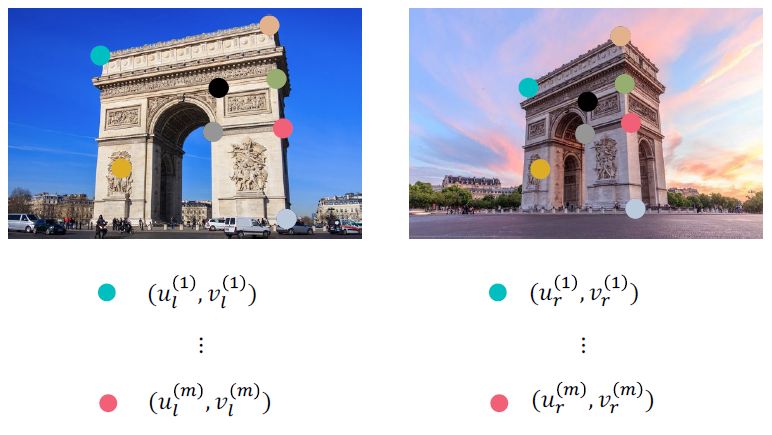
Step 1. Find a set (\(m\) pairs) of corresponding features. 找到一组(\(m\) 对)匹配点.
Least Number of Points
At least 8 pairs: \((u_l^{(i)}, v_l^{(i)})\) ↔ \((u_r^{(i)}, v_r^{(i)})\)
NOTE that one pair only corresponds one equation. (not the same as before)
Step 2. Build linear systems and solve for \(F\). 建立方程组并求解矩阵 \(F\).
For each matching \(i\),
\[
\begin{bmatrix}
u_l^{(i)} & v_l^{(i)} & 1
\end{bmatrix}
\begin{bmatrix}
f_{11} & f_{12} & f_{13} \\
f_{21} & f_{22} & f_{23} \\
f_{31} & f_{32} & f_{33}
\end{bmatrix}
\begin{bmatrix}
u_r^{(i)} \\ v_r^{(i)} \\ 1
\end{bmatrix}
= 0.
\]
Unfold it and we have
\[
\left( f_{11} u_r^{(i)} + f_{12} v_r^{(i)} + f_13 \right)u_l^{(i)} +
\left( f_{21} u_r^{(i)} + f_{22} v_r^{(i)} + f_23 \right)v_l^{(i)} +
f_{31} u_r^{(i)} + f_{32} v_r^{(i)} + f_33 = 0.
\]
For all selected points, we have
\[
\begin{bmatrix}
u_l^{(1)}u_r^{(1)} & u_l^{(1)}v_r^{(1)} & u_l^{(1)} & v_l^{(1)}u_r^{(1)} & v_l^{(1)}v_r^{(1)} & v_l^{(1)} & u_r^{(1)} & v_r^{(1)} & 1 \\
\vdots & \vdots & \vdots & \vdots & \vdots & \vdots & \vdots & \vdots & \vdots \\
u_l^{(i)}u_r^{(i)} & u_l^{(i)}v_r^{(i)} & u_l^{(i)} & v_l^{(i)}u_r^{(i)} & v_l^{(i)}v_r^{(i)} & v_l^{(i)} & u_r^{(i)} & v_r^{(i)} & 1 \\
\vdots & \vdots & \vdots & \vdots & \vdots & \vdots & \vdots & \vdots & \vdots \\
u_l^{(m)}u_r^{(m)} & u_l^{(m)}v_r^{(m)} & u_l^{(m)} & v_l^{(m)}u_r^{(m)} & v_l^{(m)}v_r^{(m)} & v_l^{(m)} & u_r^{(m)} & v_r^{(m)} & 1 \\
\end{bmatrix}
\begin{bmatrix}
f_{11} \\ f_{12} \\ f_{13} \\
f_{21} \\ f_{22} \\ f_{23} \\
f_{31} \\ f_{32} \\ f_{33} \\
\end{bmatrix}
=
\begin{bmatrix}
0 \\ 0 \\ 0 \\ 0 \\ 0 \\ 0 \\ 0 \\ 0 \\ 0
\end{bmatrix}.
\]
\[
A \mathbf{f} = \mathbf{0}.
\]
Similarly, we can give some constraints.
- Option 1. \(f_{33} = 1\).
- Option 2. \(||f|| = 1\).
Thus the degree of freedom is \(8\),at least \(8\) pairs of points.
Similarly we need to minimize \(||\mathbf{Af - 0}|| = \mathbf{||Af||}\).
And also, if we select the constraint that the vector norm is \(1\), then we only need to determine the direction of \(\mathbf{p}\), denoted by \(\mathbf{\hat p}\), and \(\mathbf{\hat p}\) is the corresponding eigenvector of the eigenvalue of \(\mathbf{A^{T}A}\).
Step 3. Find \(E\) and Extract \(R\), \(\mathbf{t}\)
\[
E = K_l^T F K_r.
\]
By SVD decomposition, from \(E = T_\times R\) we get \(T_\times\) 和 \(R\).
\(R\) is the rotation matrix and \(\mathbf{t}\) can be solved directly by \(T_\times\).
Step 4. Find 3D Position of Scene Points
Now we have
\[
\begin{aligned}
\text{Left Camera}
\\
\begin{bmatrix}
u_l \\ v_l \\ 1
\end{bmatrix}
&=
\begin{bmatrix}
f_x^{(l)} & 0 & o_x^{(l)} & 0 \\
0 & f_y^{(l)} & o_y^{(l)} & 0 \\
0 & 0 & 1 & 0
\end{bmatrix}
\begin{bmatrix}
x_l \\ y_l \\ z_l \\ 1
\end{bmatrix}
,\ \
\begin{bmatrix}
x_l \\ y_l \\ z_l \\ 1
\end{bmatrix}
=
\begin{bmatrix}
r_{11} & r_{12} & r_{13} & t_x \\
r_{21} & r_{22} & r_{23} & t_y \\
r_{31} & r_{32} & r_{33} & t_z \\
0 & 0 & 0 & 1
\end{bmatrix}
\begin{bmatrix}
x_r \\ y_r \\ z_r \\ 1
\end{bmatrix},
\\
\begin{bmatrix}
u_l \\ v_l \\ 1
\end{bmatrix}
&=
\begin{bmatrix}
f_x^{(l)} & 0 & o_x^{(l)} & 0 \\
0 & f_y^{(l)} & o_y^{(l)} & 0 \\
0 & 0 & 1 & 0
\end{bmatrix}
\begin{bmatrix}
r_{11} & r_{12} & r_{13} & t_x \\
r_{21} & r_{22} & r_{23} & t_y \\
r_{31} & r_{32} & r_{33} & t_z \\
0 & 0 & 0 & 1
\end{bmatrix}
\begin{bmatrix}
x_r \\ y_r \\ z_r \\ 1
\end{bmatrix}.
\\ \\
\normalsize
\mathbf{\tilde u}_l &=
\normalsize
P_l \mathbf{\tilde x}_r.
\\ \\
\small
\text{Right Camera}
\\
\begin{bmatrix}
u_r \\ v_r \\ 1
\end{bmatrix}
&=
\begin{bmatrix}
f_x^{(r)} & 0 & o_x^{(r)} & 0 \\
0 & f_y^{(r)} & o_y^{(r)} & 0 \\
0 & 0 & 1 & 0
\end{bmatrix}
\begin{bmatrix}
x_r \\ y_r \\ z_r \\ 1
\end{bmatrix},
\\ \\
\normalsize
\mathbf{\tilde u}_l &=
\normalsize
M_{int_r} \mathbf{\tilde x}_r.
\end{aligned}
\]
From
\[
\begin{bmatrix}
u_r \\ v_r \\ 1
\end{bmatrix}
=
\begin{bmatrix}
m_{11} & m_{12} & m_{13} & m_{14} \\
m_{21} & m_{22} & m_{23} & m_{24} \\
m_{31} & m_{32} & m_{33} & m_{34} \\
\end{bmatrix}
\begin{bmatrix}
x_r \\ y_r \\ z_r \\ 1
\end{bmatrix}
,\ \
\begin{bmatrix}
u_r \\ v_r \\ 1
\end{bmatrix}
=
\begin{bmatrix}
p_{11} & p_{12} & p_{13} & p_{14} \\
p_{21} & p_{22} & p_{23} & p_{24} \\
p_{31} & p_{32} & p_{33} & p_{34} \\
\end{bmatrix}
\begin{bmatrix}
x_r \\ y_r \\ z_r \\ 1
\end{bmatrix},
\]
we have
\[
\underbrace{
\begin{bmatrix}
u_r m_{31} - m_{11} & u_r m_{32} - m_{12} & u_r m_{33} - m_{13} \\
v_r m_{31} - m_{21} & v_r m_{32} - m_{22} & v_r m_{33} - m_{23} \\
u_l p_{31} - p_{11} & u_l p_{32} - p_{12} & u_l p_{33} - p_{13} \\
v_l p_{31} - p_{21} & v_l p_{32} - p_{22} & v_l p_{33} - p_{23}
\end{bmatrix}
}_{A_{4\times 3}}
\underbrace{
\begin{bmatrix}
x_r \\ y_r \\ z_r
\end{bmatrix}
}_{\mathbf{x}_r}
=
\underbrace{
\begin{bmatrix}
m_{14} - m_{34} \\
m_{24} - m_{34} \\
p_{14} - p_{34} \\
p_{24} - p_{34}
\end{bmatrix}
}_{\mathbf{b}}
\]
From the uniqueness of analysis, theoretically there are two rows that are linearly dependent. But in actual point selection, there can be some error, thus for maximize the usage of the data, we still use MSE.
From MSE, we have
\[
\mathbf{x}_r = (A^TA)^{-1}A^T \mathbf{b}.
\]
Non-linear Solution
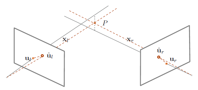
The method above is to solve linear system. And another idea is to minimize reprojection error (重映射误差).
\[
\text{cost}(P) = \text{dist}(\mathbf{u}_l, \mathbf{\hat u}_l)^2 + \text{dist}(\mathbf{u}_r, \mathbf{\hat u}_r)^2.
\]
By the way, we can optimize \(R\) and \(\mathbf{t}\) by this method.
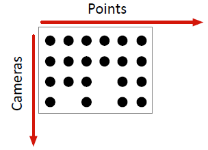
Multi-frame Structure from Motion
Similar to Two-frame SfM, given \(m\) images, \(n\) 3D points and the intrinsic matrices, find the camera pose and the 3D coordinates of the objects.
Namely for the equations below,
\[
\mathbf{u}_j^{(i)} = P_{proj}^{(i)} \mathbf{P}_j
,\ \ \text{ where } i = 1, \dots, m, j = 1, \dots, n.
\]
and \(mn\) 2D projection points \(\mathbf{u}_j^{(i)}\), find \(m\) projection matrices \(P_{proj}^{(i)}\) and 3D coordinates of \(n\) points \(P_j\).
Solution: Sequential Structrue from Motion
Step 1. Initialize camera motion and scene structure. 初始化
First, select two images to do Two-frame SfM.
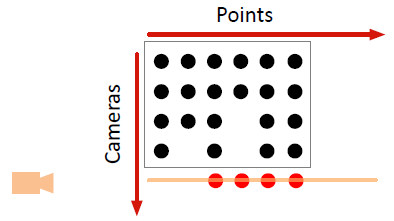
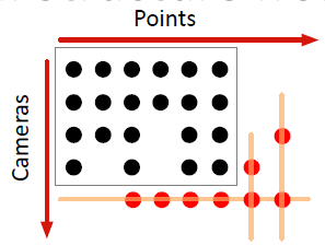
Step 2. Deal with an addition view. 处理下一张图
For each additional image,
- For the points without built 3D points: do Two-frame SfM.
Step 3. Refine structure and motion: Bundle Adjustment. 集束调整
After processing all images, we optimize the 3D coordinates and camera parameters by Bundle Adjustment (集束调整)(implemented by LM algorithm), namely optimizing reprojection error (non-linear MSE):
\[
E(P_{proj}, \mathbf{P}) = \sum\limits_{i=1}^m \sum\limits_{j=1}^n \text{dist} \left( u_j^{(i)}, P_{proj}^{(i)} \mathbf{P}_j \right)^2.
\]
COLMAP
COLMAP is a general-purpose Structure-from-Motion (SfM) and Multi-View Stereo (MVS) pipeline with a graphical and commandline interface. It offers a wide range of features for reconstruction of ordered and unordered image collections.
最后更新:
2023.11.21 17:00:13 CST
创建日期:
2022.11.10 01:04:43 CST