Fundamentals of Quantum Information¶

Quantum information science and engineering (QISE).

Lecture 1 | Information, Entropy and Computational Complexity¶

Information Entropy¶

Shannon Entropy

If $X$ is a random variable over a sete of events $x$ such that event $x$ occurs with probability $p_x$, then the Shannon entropy of event $x$ is $-\log_2(p_x)$.

If we consider a set of possible events whose probabilities of occurrence are $p_1$, $p_2$, $\dots$, $p_n$, then the average information is

\[ H = \langle I(p_i) \rangle \sim - \sum\limits_{i = 1}^{n} p_i \log_2 p_i. \]

Suppose a set of data to be compressed by a random variable $X$, for an arbitrary sequence $X_1$, $X_2$, $\dots$, $X_n$, the information of it is

\[ -\log_2 P(X_1, \dots, X_n) = -nH(X) \]

where $H(X)$ is the average information of one element. Thus

\[ P(X_1, \dots, X_n) = 2^{-nH(X)}, \]

which shows that there are at most $2^{nH(X)}$ sequences (suppose each sequence has the same probability), and hence **it only requires $nH(X)$ bits to encode them.

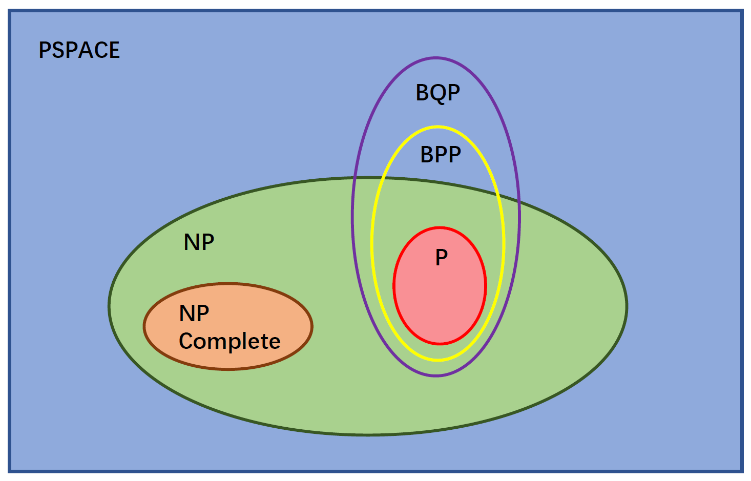
Computational Complexity¶

P, NP, BPP, BQP

In some cases, quantum algorithm can do better than classical algorithm at the computational complexity. A example is Peter Shor algorithm, which solving it in $O(n^3)$, faster than classical $2^{O(n^{1/3})}$ of an $n$-bit integer.

Lecture 2 | Dirac's Bracket and Polarization¶

Introduction

Classical systems are represented by real numbers, or maybe real vector spaces. In some cases like discussing RC circuits, we use complex numbers to simplify the procedure. However, quantum mechanics, on the other hand, is founded intrinsically on complex vector spaces.

Dirac's Bracket Notation¶

A complex vector space is composed of elements $\ket{a}$ called kets. They are column vectors in our usual notation. It has a dual space whose elements are bras $\bra{a}$.
- If $\ket{a} = (\alpha_0, \dots, \alpha_n)$, where $\alpha_i \in \mathbb{C}$, then $\bra{a} = (\alpha_0^*, \dots^*, \alpha_n^*)^T$. where $\alpha^*$ is the conjugate of $\alpha$.
Inner product $\braket{a|b}$ generalizes the dot product of usual vectors. Note that $\braket{a|b} = \braket{b|a}^*$.
Choosing an orthonormal basis of $\ket{i}$, we can expand an arbitrary $\ket{a}$ as

$$ \ket{a} = \sum\limits_{i} \ket{i}\braket{i|a}. $$ - The matrix

$$ P_i = \ket{i}\bra{i} $$ is called a projection operator (or projector) in the direction $\ket{i}$.

Polarization of Light

Review the polarization of light, we can represent linear polarization along $x$ and $y$ axis by

\[ \ket{h} = \begin{pmatrix} 1 \\ 0 \end{pmatrix}, \ket{v} = \begin{pmatrix} 0 \\ 1 \end{pmatrix}. \]

A photon in any polarization can be represented by a state $\ket{p}$

\[ \ket{p} = I\ket{p} = \ket{h}\braket{h|p} + \ket{v}\braket{v|p} = \mu \ket{h} + \nu \ket{v}, \]

where $\mu, \nu \in \mathbb{C}$ are probability amplitudes and $\braket{p|p} = \mu^2 + \nu^2 = 1$.

When measured by polarizers, probability of polarization alog $x$ and $y$ axis are

\[ P_h = \mu^2 = \braket{p|h}\braket{h|p} = \braket{p|P_h|p}, P_v = \mu^2 = \braket{p|v}\braket{v|p} = \braket{p|P_v|p}. \]

Lecture 3 | Spins, Qubits and Linear Operators¶

Stern-Gerlach Experiment

In the Stern-Gerlach experiment, a narrow beam of silver atoms passes through an electromagnet field and then lands on a glass detector plate. When the electromagnet was turned on, Stern and Gerlach found that the silver atoms formed two distinct spots on the glass plate. This experiment verifies the quantization of angular momentum.

Qubit¶

Like the polarization example in Lecture 2, the isolated quantum spin in Stern-Gerlach experiment is another realization of two-level system which we call quantum bits, or qubit.

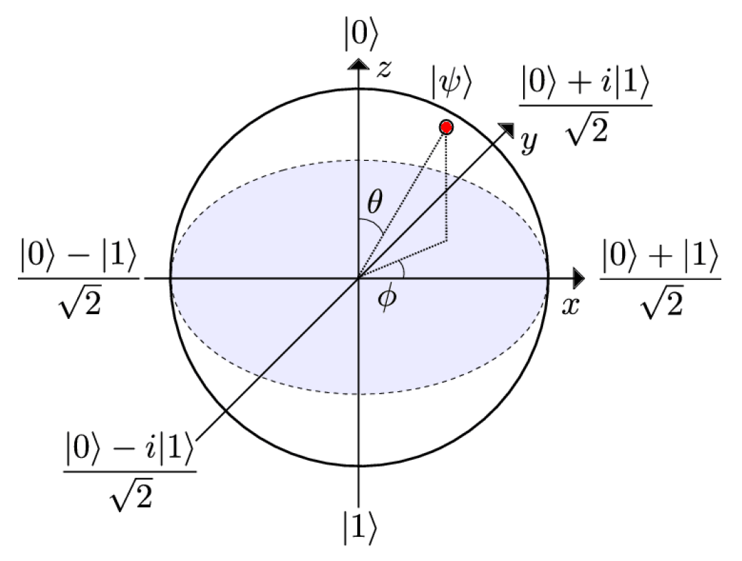
A general state of a qubit is

\[ \ket{\psi} = \alpha\ket{0} + \beta\ket{1} = \begin{pmatrix} \alpha \\ \beta \end{pmatrix},\ \ \alpha, \beta \in \mathbb{C} \]

normalized by

\[ \braket{\psi|\psi} = \alpha^2 + \beta^2 = 1. \]

We can parameterize it by

\[ \ket{\psi} = \cos\frac{\theta}{2}\ket{0} + e^{i\phi}\sin\frac{\theta}{2}\ket{1} \]

and represent it by a point on the Bloch sphere.

Linear Operator¶

Linear Operator

A map $M: \mathbb{C}^n \rightarrow \mathbb{C}^n$ is a linear operator if

\[ M(\mu\ket{x} + \nu\ket{y}) = \mu M\ket{x} + \nu M \ket{y} \]

is satisfied for arbitrary $\ket{x}, \ket{y} \in \mathbb{C}^n$ and $\mu, \nu \in \mathbb{C}$.

When we choose a set of N orthonormal $\ket{i}$, we can symbolically represent linear operator by an $N \times N$ matrix.

Hermitian Operator

If a linear operator $M$ satisfies

\[ M = M^{\dagger} = \left(M^T\right)^*. \]

Eigenvalues and Eigenvectors¶

Eigenvalues and Eigenvectors

If there is a ket-vector $\ket{\lambda}$ such that

\[ M\ket{\lambda} = \lambda\ket{\lambda}, \]

then $\lambda$ is called eigenvalue, while $\ket{\lambda}$ is called eigenvector.

Note that $M$ can be represented by its eigenvalues and eigenvectors, called spectral decomposition.

\[ M = \sum\limits_{\lambda\lambda'} \ket{\lambda} \braket{\lambda | M | \lambda'} \bra{\lambda'} = \sum\limits_{\lambda}\ket{\lambda}\bra{\lambda} = \sum\limits_{\lambda}\lambda P_\lambda. \]

Principle of Quantum Mechanics¶

Here are some principles, or say axioms of quantum mechanics.

Principle

States of a system are represented by vectors in a complex vector space.
The observables or measurable quantities of quantum mechanics are represented by linear operators $L$.
The possible results of a measurement are the eigenvalues $\lambda$ of the operator that represents the observable.
Unambiguously distinguishable states are represented by orthogonal vectors.
If $\ket{\psi}$ is a state-vector, and the observable $L$ is measured, the probability to observe $\lambda$ i

\[ P_\lambda = \braket{\psi|\lambda}\braket{\lambda|\psi} = \braket{\psi|P_\lambda|\psi}, \]

where $\ket{\lambda}$ is the corresponding eigenvector.

Pauli Matrices¶

The spin operators in the Stern-Glarch experiment is called Pauli matrices, represented by

\[ \sigma_x = \begin{pmatrix} 0 & 1 \\ 1 & 0 \end{pmatrix},\ \ \sigma_y = \begin{pmatrix} 0 & -i \\ i & 0 \end{pmatrix},\ \ \sigma_z = \begin{pmatrix} 1 & 0 \\ 0 & -1 \end{pmatrix}. \]

Their eigenvalues are all $\pm 1$.

In our classical representation, a spin is a 3D vector, but in the quantum state of a spin is a 2D complex vector. To connect with these two concepts, we use a special representation.

\[ \vec{\sigma} = \sigma_x \hat{x} + \sigma_y \hat{y} + \sigma_z \hat{z}, \]

For the spin along an arbitrary direction $\hat{n} = (n_x, n_y, n_z)$, the operator is

\[ \sigma_n = \vec{\sigma} \cdot \hat{n} = \sigma_xn_x +\sigma_yn_y + \sigma_zn_z = \begin{pmatrix} n_z & n_x - in_y \\ n_x + in_y & -n_z \end{pmatrix} \]

Lecture 4 | Quantum Entanglement¶

We represent one bit by $\ket{0} = \begin{pmatrix} 1 \\ 0 \end{pmatrix}$ and $\ket{0} = \begin{pmatrix} 0 \\ 1 \end{pmatrix}$, intuitively, we want to represent the two bit states by

\[ \ket{00} = \begin{pmatrix} 1 \\ 0 \\ 0 \\ 0 \end{pmatrix},\ \ \ket{01} = \begin{pmatrix} 0 \\ 1 \\ 0 \\ 0 \end{pmatrix},\ \ \ket{10} = \begin{pmatrix} 0 \\ 0 \\ 1 \\ 0 \end{pmatrix},\ \ \ket{11} = \begin{pmatrix} 0 \\ 0 \\ 0 \\ 1 \end{pmatrix}. \]

To meet our intuition, here is tensor product.

Tensor Product

The tensor product of an $m \times n$ matrix $A$ and a $p \times q$ matrix $B$ is an $mp \times nq$ matrix in the form

\[ A \otimes B = \begin{pmatrix} a_{11}B & a_{12}B & \cdots & a_{1n}B \\ a_{21}B & a_{22}B & \cdots & a_{2n}B \\ \vdots & \vdots & \ddots & \vdots \\ a_{n1}B & a_{n2}B & \cdots & a_{nn}B \end{pmatrix} \]

For two vector $\ket{u}$ and $\ket{v}$, we often use abbrevation as $\ket{u}\ket{v}$ or just $\ket{uv}$.

Entanglement¶

Suppose we have two qubit in $\alpha_1\ket{0} + \beta_1\ket{1}$ and $\alpha_2\ket{0} + \beta_2\ket{1}$ respectively. Then the product state is

\[ (\alpha_1\ket{0} + \beta_1\ket{1})\otimes(\alpha_2\ket{0} + \beta_2\ket{1}) = \alpha_1\alpha_2\ket{00} + \alpha_1\beta_2\ket{01} + \beta_1\alpha_2\ket{10} + \beta_1\beta_2\ket{11}. \]

If we consider each qubit respectively, we need 2 real number parameters to specify each, thus totally 4. But for the most general 2-qubit state, we need 6. This means there still some states that product states cannot represent, which is the entangled state.

A typical entangle state is Bell states, one of which is

\[ \ket{\Psi} = \frac{1}{\sqrt{2}}(\ket{01} + \ket{10}). \]

Expectation¶

Suppose an observable $L$ with eigenvalues $\lambda$, for an arbitrary state $\ket{\psi}$, we have

\[ \ket{\psi} = \sum_{\lambda} \ket{\lambda}\braket{\lambda|\psi}. \]

Act $L$ on $\ket{\psi}$,

\[ L\ket{\psi} = \sum_\lambda L\ket{\lambda}\braket{\lambda|\psi} = \sum_\lambda \lambda\ket{\lambda}\braket{\lambda|\psi}. \]

The expectation value of $L$ of the system is defined as

\[ \braket{L} = \braket{\psi|L|\psi} = \sum_\lambda \lambda\braket{\psi|\lambda}\braket{\lambda|\psi} = \sum_\lambda \lambda P(\lambda). \]

This is *the weighted sum of $L$'s eigenvalues $\lambda$ with probability $P(\lambda) = \braket{\psi|\lambda}\braket{\lambda|\psi}$.

However, we can't get any information from Bell states, since if one measures the first qubit in the Bell state, the result is $\braket{(\vec{\sigma} \cdot \hat{n}) \otimes I}$ = 0. Thus we need another ways to get the information of the entangled states.

Density Matrix¶

For pure state $\ket{\psi}$, the expectation of an operator $L$ is

\[ \braket{L} = \sum_i \braket{\psi|L|i}\braket{i|\psi} = \sum_i\braket{i|\psi}\braket{\psi|L|i} = \text{Tr}(\ket{\psi}\bra{\psi}L) = \text{Tr}\rho L, \]

where $\rho = \ket{\psi}\bra{\psi}$ is the density matrix.

For mixed state, with each state $\ket{\psi_i}$ of probability $P_i$, the density matrix is

\[ \rho = \sum_i P_i \ket{\psi_i}\bra{\psi_i}. \]

Reduced Density¶

For a separable state $\ket{\psi} = \ket{\lambda}_A\ket{\phi}_B$, the density matrix is

\[ \rho_{AB} = \ket{\psi}\bra{\psi} = \ket{\lambda}\bra{\lambda} \otimes \ket{\phi}\bra{\phi} = \rho_A \otimes \rho_B. \]

In this case, we define reduce density matrices

\[ \rho_A = \ket{\lambda}\bra{\lambda},\ \ \rho_B = \ket{\phi}\bra{\phi}. \]

Informally, the reduce density matrix of subsystem $A$ is given by

\[ \rho_A = \text{Tr}_B(\rho_{AB}). \]

Here, $\text{Tr}_B$ is partial trace, defined as

\[ \text{Tr}_B(\ket{\xi_u}\bra{\xi_v} \otimes \ket{\chi_u}\bra{\chi_v}) = \ket{\xi_u}\bra{\xi_v} \text{Tr}(\ket{\chi_u}\bra{\chi_v}), \]

where $\ket{\xi_u}$ and $\ket{\xi_v}$ are arbitrary states in $A$ and $\ket{\chi_u}$ and $\ket{\chi_v}$ are arbitrary states in $B$.

Remains

Examples.

Entanglement Entropy

To measure the entanglement of the two subsystems quantitatively, we define entanglement entropy by

\[ S_A = - \text{Tr}_A(\rho_A \log_2 \rho_A) = - \sum_i \lambda_i \log_2 \lambda_i, \]

where $\lambda_i$ are the eigenvalues of $\rho_A$.

Lecture 5 | Time Evolution of Closed Quantum Systems¶

最后更新: 2023.09.23 14:49:31 CST
创建日期: 2023.09.23 14:49:31 CST