Chapter 4 | Numerical Differentiation and Integration
Before everything start, it's necessary to introduce an approach to reduce truncation error: Richardson's extrapolation.
Richardson's Extrapolation 外推
Suppose for each \(h\), we have a formula \(N(h)\) to approximate an unknown value \(M\). And suppose the truncation error have the form
for some unknown constants \(K_1\), \(K_2\), \(K_3\), \(\dots\). This has \(O(h)\) approximation.
First, we try to make some transformation to reduce the \(K_1 h\) term.
Eliminate \(h\), and we have
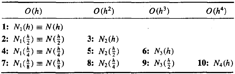
Define \(N_1(h) \equiv N(h)\) and
Then we have \(O(h^2)\) approximation formula for \(M\):
Repeat this process by eliminating \(h^2\), and then we have
where
We can repeat this process recursively, and finally we get the following conclusion.
Richardson's Extrapolation
If \(M\) is in the form
then for each \(j = 2, 3, \dots, m\), we have an \(O(h^j)\) approximation of the form
Also it can be used if the truncation error has the form
Numerical Differentiation
First Order Differentiation
Suppose \(\{x_0, x_1, \dots, x_n\}\) are distinct in some interval \(I\) and \(f \in C^{n + 1}(I)\), then we have the Lagrange interpolating polynomials,
Differentiate \(f(x)\) and substitute \(x_j\) to it,
which is called an (n + 1)-point formula to approximate \(f'(x_j)\).
For convenience, we only discuss the equally spaced situation. Suppose the interval is \([a, b]\) divided to \(n\) parts, and denote
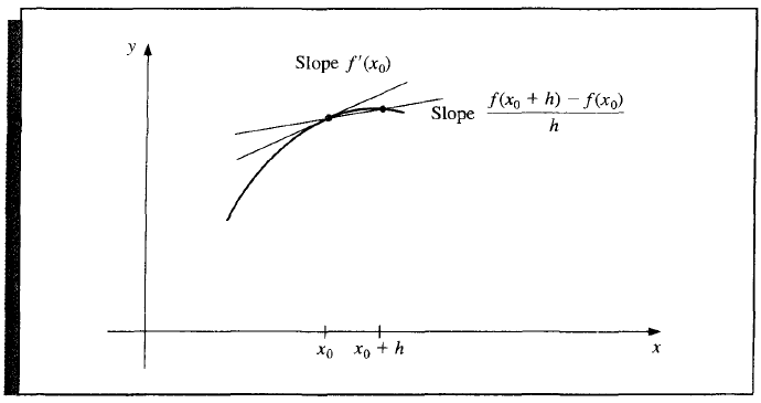
When \(n = 1\), we simply get the two-point formula,
which is known as forward-difference formula. Inversely, by replacing \(h\) with \(-h\),
is known as backward-difference formula.
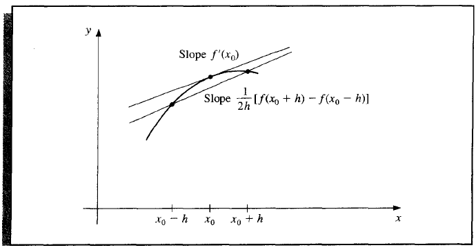
When \(n = 3\), we get the three-point formulae. Due to symmetry, there are only two.
When \(n = 5\), we get the five-point formulae. The following are the useful two of them.
Differentiation with Richardson's Extrapolation
Consider the three-point formula,
In this case, considering Richardson's extrapolation, we have
Eliminate \(h^2\), we have
where
Continuing this procedure, we have,
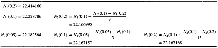
Example
Suppose \(x_0 = 2.0\), \(h = 0.2\), \(f(x) = xe^x\), the exact value of \(f'(x_0)\) is 22.167168. While the extrapolation process is shown below.
Higher Differentiation
Take second order differentiation as an example. From Taylor polynomial about point \(x_0\), we have
where \(x_0 - h < \xi_{-1} < x_0 < \xi_1 < x_0 + h\).
Add these equations and take some transformations, we get
where \(x_0 - h < \xi < x_0 + h\), and \(f^{(4)}(\xi) = \dfrac{1}{2}(f^{(4)}(\xi_1) + f^{(4)}(\xi_{-1}))\).
Error Analysis
Now we examine the formula below,
Suppose that in evaluation of \(f(x_0 + h)\) and \(f(x_0 - h)\), we encounter roundoff errors \(e(x_0 + h)\) and \(e(x_0 - h)\). Then our computed values \(\tilde f(x_0 + h)\) and \(\tilde f(x_0 - h)\) satisfy the following formulae,
Thus the total error is
Moreover, suppose the roundoff error \(e\) are bounded by some number \(\varepsilon > 0\) and \(f^{(3)}(x)\) is bounded by some number \(M > 0\), then
Thus theoretically the best choice of \(h\) is \(\sqrt[3]{3\varepsilon / M}\). But in reality we cannot compute such an \(h\) since we know nothing about \(f^{(3)}(x)\).
In all, we should aware that the step size \(h\) cannot be too large or too small.
Numerical Integration
Numerical Quadrature
Similarly to the differentiation case, suppose \(\{x_0, x_1, \dots, x_n\}\) are distinct in some interval \(I\) and \(f \in C^{n + 1}(I)\), then we have the Lagrange interpolating polynomials,
Integrate \(f(x)\) and we get
where
Definition 4.0
The degree of accuracy, or say precision, of a quadrature formula is the largest positive integer \(n\) such that the formula is exact for \(x^k\), for each \(k = 0, 1, \dots, n\).
Similarly, we suppose equally spaced situation here again.
Theorem 4.0 | (n + 1)-point closed Newton-Cotes formulae
Suppose \(x_0 = a\), \(x_n = b\), and \(h = (b - a) / n\), then \(\exists\ \xi \in (a, b)\), s.t.
if \(n\) is even and \(f \in C^{n + 2}[a, b]\), and
if \(n\) is odd and \(f \in C^{n + 1}[a, b]\),
where
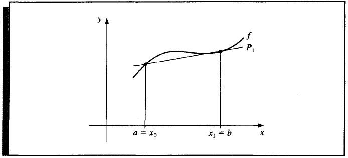
\(n = 1\) Trapezoidal rule
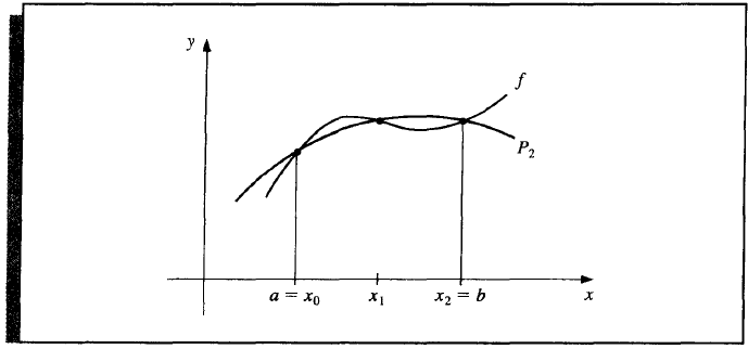
\(n = 2\) Simpson's rule
\(n = 3\) Simpson's Three-Eighths rule
Theorem 4.1 | (n + 1)-point open Newton-Cotes formulae
Suppose \(x_{-1} = a\), \(x_{n + 1} = b\), and \(h = (b - a) / (n + 2)\), then \(\exists\ \xi \in (a, b)\), s.t.
if \(n\) is even and \(f \in C^{n + 2}[a, b]\), and
if \(n\) is odd and \(f \in C^{n + 1}[a, b]\),
where
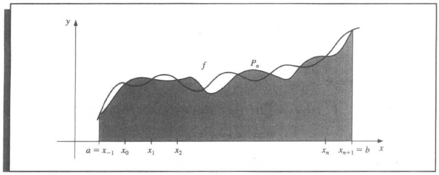
\(n = 0\) Midpoint rule
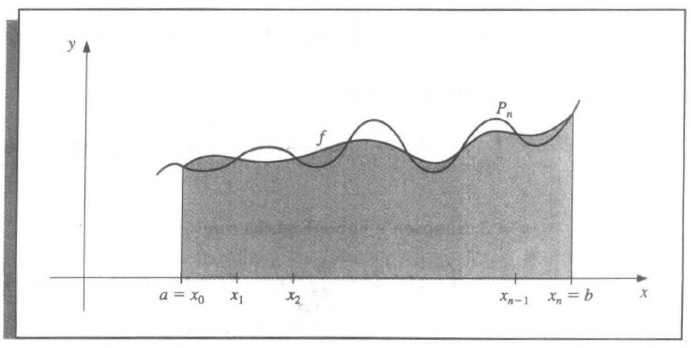
Composite Numerical Integration
Motivation: Although the Newton-Cotes gives a better and better approximation as \(n\) increases, since it's based on interpolating polynomials, it also owns the oscillatory nature of high-degree polynomials.
Similarly, we discuss a piecewise approach to numerical integration with low-order Newton-Cotes formulae. These are the techniques most often applied.
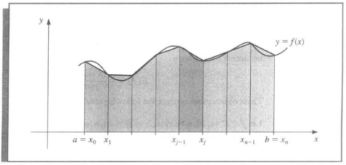
Theorem 4.2 | Composite Trapezoidal rule
\(f \in C^2[a, b]\), \(h = (b - a) /n\), and \(x_j = a + jh\), \(j = 0, 1, \dots, n\). Then \(\exists\ \mu \in (a, b)\), s.t.
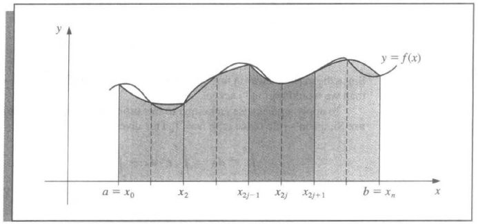
Theorem 4.3 | Composite Simpson's rule
\(f \in C^2[a, b]\), \(h = (b - a) /n\), and \(x_j = a + jh\), \(j = 0, 1, \dots, n\). Then \(\exists\ \mu \in (a, b)\), s.t.
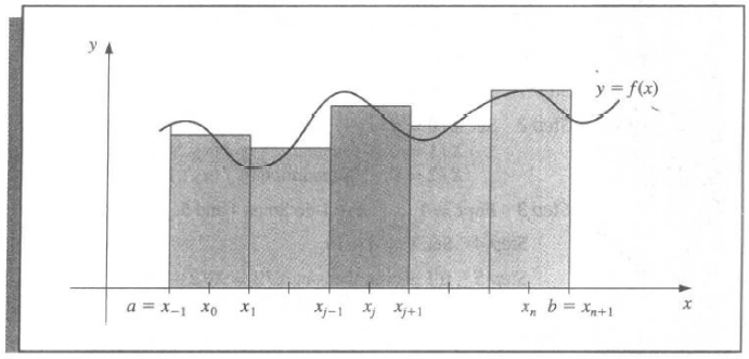
Theorem 4.4 | Composite Midpoint rule
\(f \in C^2[a, b]\), \(h = (b - a) / (n + 2)\), and \(x_j = a + (j + 1)h\), \(j = -1, 0, \dots, n + 1\). Then \(\exists\ \mu \in (a, b)\), s.t.
Stability
Composite integration techniques are all stable w.r.t roundoff error.
Example: Composite Simpson's rule
Suppose \(f(x_i)\) is apporximated by \(\tilde f(x_i)\) with
Then the accumulated error is
Suppose \(e_i\) are uniformly bounded by \(\varepsilon\), then
That means even though divide an interval to more parts, the roundoff error will not increase, which is quite stable.
Romberg Integration
Romberg integration combine the Composite Trapezoidal rule and Richardson's extrapolation to derive a more useful approximation.
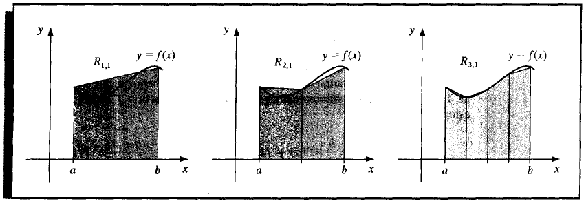
Suppose we divide the interval \([a, b]\) into \(m_1 = 1\), \(m_2 = 2\), \(\dots\), and \(m_n = 2^{n - 1}\) subintervals respectively. For each division, then the step size \(h_k\) is \((b - a) / m_k = (b - a) / 2^{k - 1}\).
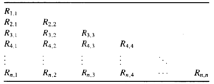
Then we use \(R_{k, 1}\) to denote the composite trapezoidal rule,
Mathematically, we have the recursive formula,
Theorem 4.5
the Composite Trapezoidal rule can represented by an alternative error term in the form
where \(K_i\) depends only on \(f^{(2i-1)}(a)\) and \(f^{(2i-1)}(b)\).
This nice theorem makes Richardson's extrapolation available to reduce the truncation error! Similar to Differentiation with Richardson's Extrapolation, we have the following formula.
Romberg Integration
with an \(O(h^{2j}_k)\) approximation.
Adaptive Quadrature Methods
Motivation: On the premise of equal spacing, in some cases, the left half of the interval is well approximated, and maybe we only need to subdivide the right half to approximate better. Here we introduce the Adaptive quadrature methods based on the Composite Simpson's rule.
First, we want to derive, if we apply Simpson's rule in two subinterval and add them up, how much precision does it improve compared to only applying Simpson's rule just in the whole interval.
From Simpson's rule, we have
where
If we divide \([a, b]\) into two subintervals, applying Simpson's rule respectively (namely apply Composite Simpson's rule with \(n = 4\) and step size \(h / 2\)), we have
Moreover, assume \(f^{(4)}(\mu) \approx f^{(4)}(\tilde \mu)\), then we have
so
Then,
This result means that the subdivision approximates \(\int_a^b f(x) dx\) about 15 times better than it agree with \(S(a, b)\). Thus suppose we have a tolerance \(\varepsilon\) across the interval \([a, b]\). If
then we expect to have
and the subdivision is thought to be a better approximation to \(\int_a^bf(x)dx\).
Conclusion
Suppose we have a tolerance \(\varepsilon\) on \([a, b]\), and we expect the tolerance is uniform. Thus at the subinterval \([p, q] \subseteq [a, b]\), with \(q - p = k(b - a)\), we expect the tolerance as \(k\varepsilon\).
Moreover, suppose the approximation of Simpson's rule on \([p, q]\) is \(S\) while the approxiamtion of Simpson's rule on \([p, (p + q) / 2]\) and \([(p + q) / 2, q]\) are \(S_1\) and \(S_2\) respectively.
Then the criterion to subdivide is that
where \(M\) is often taken as 10 but not 15, which we derive above, since it also consider the error between \(f^{(4)}(\mu)\) and \(f^{(4)}(\tilde \mu)\).
Gaussian Quadrature
Instead of equal spacing in the Newton-Cotes formulae, the selection of the points \(x_i\) also become variables. Gaussian Quadrature is aimed to construct a formula \(\sum\limits_{k = 0}^n A_kf(x_k)\) to approximate \(\int_a^b w(x)f(x)dx\) of precision degree \(2n + 1\) with \(n + 1\) points, where \(w(x)\) is a weight function. (Compare to the equally spaced strategy only have a precision of around \(n\)).
That means, to determine \(x_i\) and \(A_i\) (totally \(2n + 2\) unknowns) such that the formula is accurate for \(f(x) = 1, x, \dots, x^{2n + 1}\) (totally \(2n + 2\) equations). The selected points \(x_i\) are called Gaussian points.
Problem
Theoretically, since we have \(2n + 2\) unknowns and \(2n + 2\) eqautions, we can solve out \(x_i\) and \(A_i\). But the equations are not linear!
Thus we give the following theorem to find Gaussian points without solving the nonlinear eqautions. Recap the definition of weight function and orthogonality of polynomials, and the construction of the set of orthogonal polynomials.
Theorem 4.6
\(x_0, \dots, x_n\) are Gaussian point iff \(W(x) = \prod\limits_{k = 0}^n (x - x_k)\) is orthogonal to all the polynomials of degree no greater than \(n\) on interval \([a,b]\) w.r.t the weight function \(w(x)\).
Proof
\(\Rightarrow\)
if \(x_0, \dots x_n\) are Gaussian points, then the degree of precision of the formula \(\int_a^b w(x)f(x)dx \approx \sum\limits_{k = 0}^n A_k f(x_k)\) is at least \(2n + 1\).
Then \(\forall\ P(x) \in \Pi_n\), \(\text{deg}(P(x)W(x)) \le 2n + 1\). Thus
\(\Leftarrow\)
\(\forall\ P(x) \in \Pi_{2n + 1}\), let \(P(x) = W(x)q(x) + r(x),\ \ q(x), r(x) \in \Pi_{n}\), then
Recap that the set of orthogonal polynomials \(\{\varphi_0, \dots, \varphi_n, \dots\}\) is linearly independent and \(\varphi_{n + 1}\) is orthogonal to any polynomials of degree no greater than \(n\).
Thus we can take \(\varphi_{n + 1}(x)\) to be \(W(x)\) and the roots of \(\varphi_{n + 1}(x)\) are the Gaussian points.
Genernal Solution
Problem: Assume
Step.1 Construct the set of orthogonal polynomial on the interval \([a, b]\) by Gram-Schimidt Process from \(\varphi_0(x) \equiv 1\) to \(\varphi_{n}(x)\).
Step.2 Find the roots of \(\varphi_{n}(x)\), which are the Gaussian points \(x_0, \dots, x_n\).
Step.3 Solve the linear systems of the equation given by the precision for \(f(x) = 1, x, \dots, x^{2n + 1}\), and obtain \(A_0, \dots, A_n\).
Although the method above is theoretically available, but it's tedious. But we have some special solutions which have been calculated. With some transformations, we can make them to solve the general problem too.
Legendre Polynomials
A typical set of orthogonal functions is Legrendre Polynomials.
Legrendre Polynomials
or equally defined recursively by
Property
-
\(\{P_n(x)\}\) are orthogonal on \([-1, 1]\), w.r.t the weight function
\[ w(x) \equiv 1. \]\[ (P_j, P_k) = \left\{ \begin{aligned} & 0, && k \ne l, \\ & \frac{2}{2k + 1}, && k = l. \end{aligned} \right. \] -
\(P_n(x)\) is a monic polynomial of degree \(n\).
- \(P_n(x)\) is symmetric w.r.t the origin.
- The \(n\) roots of \(P_n(x)\) are all on \([-1, 1]\).
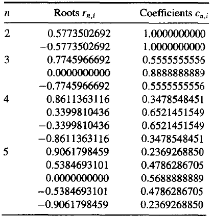
The first few of them are
The following table gives the pre-calculated values.
And from interval \([-1, 1]\) to \([a, b]\), we have a linear map
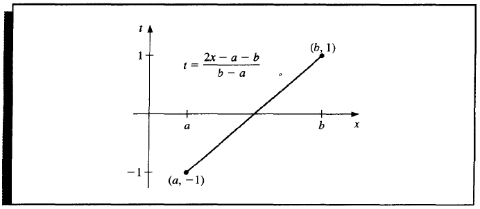
Thus we have
The formula using the roots of \(P_{n + 1}(x)\) is called the Gauss-Legendre quadrature formula.
Example
Approxiamte \(\int_1^{1.5} e^{-x^2}dx\) (exact value to 7 decimal places is 0.1093643).
Solution.
For \(n = 2\),
For \(n = 3\),
Chebyshev Polynomials
Also, Chebyshev polynomials are typical set of orthogonal polynomials too. We don't discuss much about it there.
The formula using the roots of \(T_{n + 1}(x)\) is called the Gauss-Chebyshev quadrature formula.
创建日期: 2022.11.10 01:04:43 CST