Lecture 4 Model Fitting and Optimization
Optimization
Target
- \(x \in \mathbb{R}^n\) is a vector variable to be chosen.
- \(f_0\) is the objective function to be minimized.
- \(f_1, \dots, f_m\) are the inequality constraint functions.
- \(g_1, \dots, g_p\) are the equality constraint functions.
Model Fitting
A typical approach: Minimize the Mean Square Error (MSE)
Reasons to choose MSE
Key Assumptions: MSE is MLE with Gaussian noise.
From Maximum Likelihood Estimation (MLE), the data is assumed to be with Gaussian noise.
The likelihood of observing \((a_i, b_i)\) is
If the data points are independent,
Numerical Methods
Analytical Solution 解析解
The derivative of \(||Ax-b||^2_2\) is \(2A^T(Ax - b)\), let it be \(0\). Then we get \(\hat x\) satisfying
But, if no analytical solution, we should only consider the approximate solution.
Approximate Solution 近似解
Method
- \(x \leftarrow x_0\) (Initialization),
- while not converge,
- \(p \leftarrow \text{descending\_direction(x)}\),
- \(\alpha \leftarrow \text{descending\_step(x)}\),
- \(x \leftarrow x + \alpha p\).
Gradient Descent (GD)
Steepest Descent Method
- Direction \(\Delta x = -J^T_F\).
-
Step
-
To minimize \(\phi(a)\).
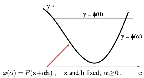
Backtracking Algorithm
- Initialize \(\alpha\) with a large value.
- Decrease \(\alpha\) until \(\phi(\alpha)\le\phi(0) + \gamma\phi'(0)\alpha\).

-
-
Advantage
- Easy to implement.
- Perform well when far from the minimum.
- Disadvantage
- Converge slowly when near the minimum, which wastes a lot of computation.
Newton Method
- Direction \(\Delta x = -H_F^{-1}J^T_F\).
- Advantage
- Faster convergence.
- Disadvantage
- Hessian matrix requires a lot of computation.
Gauss-Newton Method
For \(\hat x = \mathop{\arg\min}\limits_x ||Ax-b||^2_2 \overset{\Delta}{=\!=}\mathop{\arg\min}\limits_x||R(x)||^2_2\), expand \(R(x)\).
-
Direction \(\Delta x = -(J_R^TJ_R)^{-1}J_R^TR(x_k) = -(J_R^TJ_R)^{-1}J_F^T\)
- Compared to Newton Method, \(J_R^TJ_R\) is used to approximate \(H_F\).
-
Advantage
- No need to compute Hessian matrix.
- Faster to converge.
-
Disadvantage
- \(J^T_RJ_R\) may be singular.
Levenberg-Marquardt (LM)
-
Direction \(\Delta x = -(J_R^TJ_R + \lambda I)^{-1}J_R^TR(x_k)\).
- \(\lambda \rightarrow \infty\) Steepest Descent.
- \(\lambda \rightarrow 0\) Gauss-Newton.
-
Advantage
- Start and converge quickly.
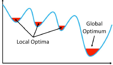
Local Minimum and Global Minimum
Convex Optimization
Remains
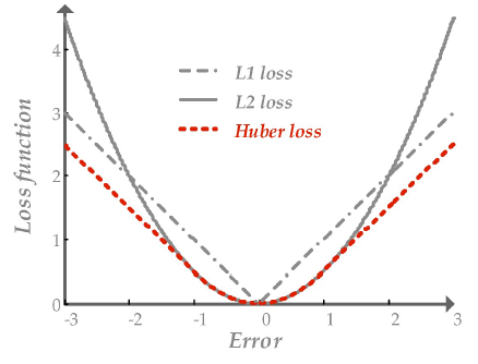
Robust Estimation
Inlier obeys the model assumption. Outlier differs significantly rom the assumption.
Outlier makes MSE fail. To reduce its effect, we can use other loss functions, called robust functions.
RANSAC (RANdom SAmple Concensus)
The most powerful method to handle outliers.
Key ideas
- The distribution of inliers is similar while outliers differ a lot.
- Use data point pairs to vote.

ill-posed Problem 病态问题 / 多解问题
Ill-posed problems are the problems that the solution is not unique. To make it unique:
-
L2 regularization
- Suppress redundant variables.
- \(\min_x||Ax-b||^2_2,\ s.t. ||x||_2 \le 1\). (the same as \(\min_x||Ax-b||^2_2 + \lambda||x||_2\))
-
L1 regularization
- Make \(x\) sparse.
- \(\min_x||Ax-b||^2_2,\ s.t. ||x||_1 \le 1\). (the same as \(\min_x||Ax-b||^2_2 + \lambda||x||_1\))
Graphcut and MRF
A key idea: Neighboring pixels tend to take the same label.
Images as Graphs
- A vertex for each pixel.
- An edge between each pair, weighted by the affinity or similarity between its two vertices.
- Pixel Dissimilarity \(S(\textbf{f}_i, \textbf{f}_j) = \sqrt{\sum_k(f_{ik} - f_{jk})^2}\).
- Pixel Affinity \(w(i, j) = A(\textbf{f}_i, \textbf{f}_j) = \exp\left(-\dfrac{1}{2\sigma^2}S(\textbf{f}_i, \textbf{f}_j)\right)\).
- Graph Notation \(G = (V, E)\).
- \(V\): a set of vertices.
- \(E\): a set of edges.
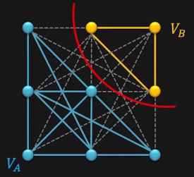
Graph Cut
Cut \(C=(V_A, V_B)\) is a parition of vertices \(V\) of a graph \(G\) into two disjoint subsets \(V_A\) and \(V_B\).
Cost of Cut: \(\text{cut}(V_A, V_B) = \sum\limits_{u\in V_A, v\in V_B} w(u, v)\).
Problem with Min-Cut
Min-cut is bias to cut small and isolated segments.

Solution: Normalized Cut
Compute how strongly verices \(V_A\) are associated with vertices \(V\).
Markow Random Field (MRF)
Graphcut is an exception of MRF.
Question
创建日期: 2022.11.09 00:35:37 CST