Chapter 7 | Iterative Techniques in Matrix Algebra

Norms of Vectors and Matrices

Vector Norms

Definition 7.0

A vector norm on \(\mathbb{R}^n\) is a function \(||\cdot||\), from \(\mathbb{R}^n\) into \(\mathbb{R}\) with the following properties.

\[ \begin{aligned} \forall \mathbf{x, y} \in \mathbb{R}^n, \alpha \in \mathbb{R}, & (1)\ ||\mathbf{x}|| \ge 0;\ ||\mathbf{x}|| = 0 \Leftrightarrow \mathbf{x} = \mathbf{0}; \\ & (2)\ ||\alpha \mathbf{x}|| = |\alpha| \cdot ||\mathbf{x}||; \\ & (3)\ ||\mathbf{x} + \mathbf{y}|| \le ||\mathbf{x}|| + ||\mathbf{y}||. \\ \end{aligned} \]

Commonly used examples

• L1 Norm: \(||\mathbf{x}||_1 = \sum\limits_{i = 1}^n|x_i|\).
• L2 Norm / Euclidean Norm: \(||\mathbf{x}||_2 = \sqrt{\sum\limits_{i = 1}^n|x_i|^2}\).
• p-Norm: \(||\mathbf{x}||_p = \left(\sum\limits_{i = 1}^n|x_i|^p\right)^{1/p}\).
• Infinity Norm: \(||\mathbf{x}||_\infty = \max\limits_{1 \le i \le n} |x_i|\).

Convergence of Vector

Definition 7.1

Similarly with a scalar, a sequence of vectors \(\{\mathbf{x}^{(k)}\}_{k=1}^\infty\) in \(\mathbb{R}^n\) is said to converge to \(\mathbf{x}\) with respect to norm \(||\cdot||\), if

\[ \forall\ \varepsilon \gt 0,\ \ \exists\ N \in \mathbb{N},\ \ \text{ s.t. } \forall\ k \gt N,\ \ ||\mathbf{x}^{(k)} - \mathbf{x}|| \lt \varepsilon. \]

Theorem 7.0

\(\{\mathbf{x}^{(k)}\}_{k=1}^\infty\) in \(\mathbb{R}^n\) converges to \(\mathbf{x}\) with respect to norm \(||\cdot||_\infty\) iff

\[ \forall\ i,\ \ \lim\limits_{k \rightarrow \infty}x_i^{(k)} = x_i. \]

Equivalence

Definition 7.2

\(||\mathbf{x}||_A\) and \(||\mathbf{x}||_B\) are equivalent, if

\[ \exists\ C_1, C_2,\ \ \text{ s.t. } C_1||\mathbf{x}||_B \le ||\mathbf{x}||_A \le C_2||\mathbf{x}||_B. \]

Theorem 7.1

All the vector norms on \(\mathbb{R}^n\) are equivalent.

Matrix Norms

Definition 7.3

A matrix norm on \(\mathbb{R}^n\) is a function \(||\cdot||\), from \(M_n(\mathbb{R})\) matrices into \(\mathbb{R}\) with the following properties.

\[ \begin{aligned} \forall A, B \in M_n(\mathbb{R}), \alpha \in \mathbb{R}, & (1)\ ||A|| \ge 0;\ ||A|| = 0 \Leftrightarrow A = \mathbf{O}; \\ & (2)\ ||\alpha A|| = |\alpha| \cdot ||A||; \\ & (3)\ ||A + B|| \le ||A|| + ||B||; \\ & (4)\ ||AB|| \le ||A|| \cdot ||B||. \end{aligned} \]

Commonly used examples

• Frobenius Norm: \(||A||_F = \sqrt{\sum\limits_{i=1}^n\sum\limits_{j=1}^n|a_{ij}|^2}\).
• Natural Norm: \(||A||_p = \max\limits_{\mathbf{x}\ne \mathbf{0}} \dfrac{||A\mathbf{x}||_p}{||\mathbf{x}||_p} = \max\limits_{||\mathbf{x}||_p = 1} ||A\mathbf{x}||_p\), where \(||\cdot||_p\) is the vector norm.
  • \(||A||_\infty = \max\limits_{1\le i \le n}\sum\limits_{j=1}^n|a_{ij}|\).
  • \(||A||_1= \max\limits_{1\le j \le n}\sum\limits_{i=1}^n|a_{ij}|\).
  • (Spectral Norm) \(||A||_2= \sqrt{\lambda_{max}(A^TA)}\).

Corollary 7.2

For any vector \(\mathbf{x} \ne 0\), matrix \(A\), and any natural norm \(||\cdot||\), we have

\[ ||A\mathbf{x}|| \le ||A|| \cdot ||\mathbf{x}||. \]

Eigenvalues and Eigenvectors

Definition 7.4 (Recap)

If \(A\) is a square matrix, the characteristic polynomial of \(A\) is defined by

\[ p(\lambda) = \text{det}(A - \lambda I). \]

The roots of \(p\) are eigenvalues. If \(\lambda\) is an eigenvalue and \(\mathbf{x} \ne 0\) satisfies \((A - \lambda I)\mathbf{x} = \mathbf{0}\), then \(\mathbf{x}\) is an eigenvector.

Spectral Radius

Definition 7.5

The spectral radius of a matrix \(A\) is defined by

\[ \rho(A) = \max|\lambda|,\ \ \text{ where $\lambda$ is an eigenvalue of $A$}. \]

(Recap that for complex \(\lambda = \alpha + \beta i\), \(|\lambda| = \sqrt{\alpha^2 + \beta^2}\).)

Theorem 7.3

\(\forall\ A \in M_n(\mathbb{R})\),

• \(||A||_2 = \sqrt{\rho(A^tA)}\).
• \(\rho(A) \le ||A||\), for any natural norm \(||\cdot||\).

Proof

A proof for the second property. Suppose \(\lambda\) is an eigenvalue of \(A\) with eigenvector \(\mathbf{x}\) and \(||\mathbf{x}|| = 1\),

\[ |\lambda| = |\lambda| \cdot ||\mathbf{x}|| = ||\lambda \mathbf{x}|| \le ||A|| \cdot ||\mathbf{x}|| = ||A||. \]

Thus,

\[ \rho(A) = \max|\lambda| \le ||A||. \]

Convergence of Matrix

Definition 7.6

\(A \in M_n(\mathbb{R}))\) is convergent if

\[ \lim_{k \rightarrow \infty}\left(A^k\right)_{ij} = 0,\ \ \text{ for each } i = 1, 2, \dots, n \text{ and } j = 1, 2, \dots, n. \]

Theorem 7.4

The following statements are equivalent.

• \(A\) is a convergent matrix.
• \(\lim\limits_{n \rightarrow \infty} ||A^n|| = 0\), for some natural norm.
• \(\lim\limits_{n \rightarrow \infty} ||A^n|| = 0\), for all natural norms.
• \(\rho(A) < 1\).
• \(\forall\ \mathbf{x}\), \(\lim\limits_{n \rightarrow \infty} ||A^n \mathbf{x}|| = \mathbf{0}\).

Iterative Techniques for Solving Linear Systems

\[ A\mathbf{x} = \mathbf{b} \Leftrightarrow (D - L - U)\mathbf{x} = \mathbf{b} \Leftrightarrow D\mathbf{x} = (L + U)\mathbf{x} + \mathbf{b} \\ \]

Thus,

\[ \mathbf{x} = D^{-1}(L + U)\mathbf{x} + D^{-1}\mathbf{b}. \]

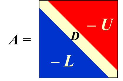
Jacobi Iterative Method

Let \(T_j = D^{-1}(L+U)\) and \(\mathbf{c}_\mathbf{j} = D^{-1}\mathbf{b}\), then

\[ \mathbf{x}^{(k)} = T_j\mathbf{x}^{(k - 1)} + \mathbf{c}_\mathbf{j}. \]

Gauss-Seidel Iterative Method

\[ \small \mathbf{x}^{(k)} = D^{-1}(L\mathbf{x}^{(k)} + U\mathbf{x}^{(k - 1)}) + D^{-1}\mathbf{b} \Leftrightarrow \mathbf{x}^{(k)} = (D - L)^{-1}U\mathbf{x}^{(k - 1)} + (D - L)^{-1}\mathbf{b} \]

Let \(T_g = (D - L)^{-1}U\) and \(\mathbf{c}_\mathbf{g} = (D - L)^{-1}\mathbf{b}\), then

\[ \mathbf{x}^{(k)} = T_g\mathbf{x}^{(k - 1)} + \mathbf{c}_\mathbf{g}. \]

Convergence

Consider the following formula

\[ \mathbf{x}^{(k)} = T\mathbf{x}^{(k - 1)} + \mathbf{c}, \]

where \(\mathbf{x}^{(0)}\) is arbitrary.

Lemma 7.5

If \(\rho(T) \lt 1\) , then \((I - T)^{-1}\) exists and

\[ (I - T)^{-1} = \sum\limits_{j = 0}^\infty T^j. \]

Proof

Suppose \(\lambda\) is an eigenvalue of \(T\) with eigenvector \(\mathbf{x}\), then since \(T\mathbf{x} = \lambda \mathbf{x} \Leftrightarrow (I - T)\mathbf{x} = (1 - \lambda)\mathbf{x}\), thus \(1 - \lambda\) is an eigenvalue of \(I - T\). Since \(|\lambda| \le \rho(T) < 1\), thus \(\lambda = 1\) is not an eigenvalue of \(T\) and \(0\) is not an eigenvalue of \(I - T\). Hence, \((I - T)^{-1}\) exists.

Let \(S_m = I + T + T^2 + \cdots + T^m\), then

\[ (I - T)S_m = (1 + T + \cdots + T^m) - (T + T^2 + \cdots + T^{m + 1}) = I - T^{m + 1}. \]

Since \(T\) is convergent, thus

\[ \lim\limits_{m \rightarrow \infty} (I - T)S_m = \lim\limits_{m \rightarrow \infty}(I - T^{m + 1}) = I. \]

Thus, \((I - T)^{-1} = \lim\limits_{m \rightarrow \infty}S_m = \sum\limits_{j = 0}^\infty T^j\).

Theorem 7.6

\(\{\mathbf{x}^{(k)}\}_{k=1}^\infty\) defined by \(\mathbf{x}^{(k)} = T\mathbf{x}^{(k - 1)} + \mathbf{c}\) converges to the unique solution of

\[ \mathbf{x} = T\mathbf{x} + \mathbf{c} \]

iff

\[ \rho(T) \lt 1. \]

Proof

\(\Rightarrow\):

Define error \(\mathbf{e}^{(k)} = \mathbf{x} - \mathbf{x}^{(k)}\), then

\[ \mathbf{e}^{(k)} = (T\mathbf{x} + c) - (T\mathbf{x}^{(k - 1)} + c) = T(\mathbf{x} - \mathbf{x}^{(k - 1)})T\mathbf{e}^{(k - 1)} \Rightarrow \mathbf{e}^{(k)} = T^k \mathbf{e}^{(0)}. \]

Since it converges, thus

\[ \lim\limits_{k \rightarrow \infty} \mathbf{e}^{(k)} = 0 \Rightarrow \forall\ \mathbf{e}^{(0)},\ \ \lim\limits_{k \rightarrow \infty} T^k \mathbf{e}^{(0)} = 0 \]

\[ \Leftrightarrow \rho(T) < 1. \]

\(\Leftarrow\):

\[ \mathbf{x}^{(k)} = T^{k}\mathbf{x}^{(0)} + (T^{k - 1} + \cdots + T + I) \mathbf{c}. \]

Since \(\rho(T) < 1\), \(T\) is convergent and

\[ \lim\limits_{k \rightarrow \infty} T^k \mathbf{x}^{(0)} = \mathbf{0}. \]

From Lemma 7.5, we have

\[ \lim\limits_{k \rightarrow \infty} \mathbf{x}^{(k)} = \lim\limits_{k \rightarrow \infty} T^k\mathbf{x}^{(0)} + \left(\sum\limits_{j = 0}^\infty T^j \right)\mathbf{c} = \mathbf{0} + (I - T)^{-1}\mathbf{c} = (I - T)^{-1}\mathbf{c}. \]

Thus \(\{\mathbf{x}^{(k)}\}\) converges to \(\mathbf{x} \equiv (I - T)^{-1} \Leftrightarrow \mathbf{x} = T\mathbf{x} + c\).

Corollary 7.7

If \(||T||\lt 1\) for any matrix norm and \(\mathbf{c}\) is a given vector, then \(\forall\ \mathbf{x}^{(0)}\in \mathbb{R}^n\) and \(\{\mathbf{x}^{(k)}\}_{k=1}^\infty\) defined by \(\mathbf{x}^{(k)} = T\mathbf{x}^{(k - 1)} + \mathbf{c}\) converges to \(\mathbf{x}\), and the following error bounds hold

• \(||\mathbf{x} - \mathbf{x}^{(k)}|| \le ||T||^k||\mathbf{x}^{(0)} - \mathbf{x}||\).
• \(||\mathbf{x} - \mathbf{x}^{(k)}|| \le \dfrac{||T||^k}{1 - ||T||}||\mathbf{x}^{(1)} - \mathbf{x}||\).

Theorem 7.8

Suppose \(A\) is strictly diagonally dominant, then \(\forall\ \mathbf{x}^{(0)}\), both Jacobi and Gauss-Seidel methods give \(\{\mathbf{x}^{(k)}\}_{k=0}^\infty\) that converge to the unique solution of \(A\mathbf{x} = \mathbf{b}\).

Relaxation Methods

Definition 7.7

Suppose \(\mathbf{\tilde x}\) is an approximation to the solution of \(A\mathbf{x} = \mathbf{b}\), then the residual vector for \(\mathbf{\tilde x}\) w.r.t this linear system is

\[ \mathbf{r} = \mathbf{b} - A\mathbf{\tilde x}. \]

Further examine Gauss-Seidel method.

\[ x_i^{(k)} = x_i^{(k - 1)} + \frac{r_i^{(k)}}{a_{ii}},\ \ \text{ where } r_i^{(k)} = b_i - \sum_{j \lt i} a_{ij}x_j^{(k)} - \sum_{j \ge i} a_{ij}x_j^{(k - 1)}. \]

Let \(x_i^{(k)} = x_i^{(k - 1)} + \omega\dfrac{r_i^{(k)}}{a_{ii}}\), by modifying the value of \(\omega\), we can somehow get faster convergence.

• \(0 \lt \omega \lt 1\) Under-Relaxation Method
• \(\omega = 1\) Gauss-Seidel Method
• \(\omega \gt 1\) Successive Over-Relaxation Method (SOR)

In matrix form,

\[ \mathbf{x}^{(k)} = (D - \omega L)^{-1}[(1 - \omega)D + \omega U]\mathbf{x}^{(k - 1)} + (D - \omega L)^{-1}\mathbf{b}. \]

Let \(T_\omega = (D - \omega L)^{-1}[(1 - \omega)D + \omega U]\) and \(\mathbf{c}_\omega = (D - \omega L)^{-1}\mathbf{b}\), then

\[ \mathbf{x}^{(k)} = T_\omega\mathbf{x}^{(k - 1)} + \mathbf{c}_\omega. \]

Theorem 7.9 (Kahan)

If \(a_{ii} \ne 0\), then \(\rho(T_\omega)\ge |\omega -1 |\), which implies that SOR method can converge only if

\[ 0 \lt \omega \lt 2. \]

Proof

Recap that upper and lower triangular determinant are equal to the product of the entries at its diagnoal.

Since \(D\) is diagonal, \(L\) and \(U\) are lower and upper triangular matrix, thus

\[ \begin{aligned} \text{det}(T_\omega) &= \text{det}((D - \omega L)^{-1}) \cdot \text{det}((1 - \omega)D + \omega U) \\ &= \text{det}(D^{-1})(1-\omega)^n\text{det}(D) = (1 - \omega)^n. \end{aligned} \]

On the other hand, recap that

\[ \text{det}(T_\omega) = \prod\limits_{i = 1}^n \lambda_i,\ \ \text{ where $\lambda_i$ are eigenvalues of $T$}. \]

Thus

\[ \rho(T_\omega) = \max\limits_{1 \le i \le n} |\lambda_i| \ge |\omega - 1|. \]

Theorem 7.10 (Ostrowski-Reich)

If \(A\) is positive definite and \(0 \lt \omega \lt 2\), the SOR method converges for any choice of initial approximation vector \(\mathbf{x}^{(0)}\).

Theorem 7.11

If \(A\) is positive definite and tridiagonal, then \(\rho(T_g) = \rho^2(T_j)\lt1\), and the optimal choice of \(\omega\) for the SOR method is

\[ \omega = \frac{2}{1 + \sqrt{1 - \rho(T_j)^2}}. \]

With this choice of \(\omega\), we have \(\rho(T_\omega) = \omega - 1\).

Error Bounds and Iterative Refinement

Definition 7.8

The conditional number of the nonsigular matrix \(A\) relative to a norm \(||\cdot||\) is

\[ K(A) = ||A|| \cdot ||A^{-1}||. \]

A matrix \(A\) is well-conditioned if \(K(A)\) is close to \(1\), and is ill-conditioned when \(K(A)\) is significantly greater than \(1\).

Proposition

• If \(A\) is symmetric, then \(K(A)_2 = \dfrac{\max|\lambda|}{\min|\lambda|}\).
• \(K(A)_2 = 1\) if \(A\) is orthogonal.
• \(\forall\ \text{ orthogonal matrix } R\), \(K(RA)_2 = K(AR)_2 = K(A)_2\).
• \(\forall\ \text{ natural norm } ||\cdot||_p\), \(K(A)_p \ge 1\).
• \(K(\alpha A) = K(A)\).

Theorem 7.12

For any natural norm \(||\cdot||\),

\[ ||\mathbf{x} - \mathbf{\tilde x}|| \le ||\mathbf{r}|| \cdot ||A^{-1}||, \]

and if \(\mathbf{x} \ne \mathbf{0}\) and \(\mathbf{b} \ne \mathbf{0}\),

\[ \frac{||\mathbf{x} - \mathbf{\tilde x}||}{||\mathbf{x}||} \le ||A||\cdot||A^{-1}|| \frac{||\mathbf{r}||}{||\mathbf{b}||} = K(A)\frac{||\mathbf{r}||}{||\mathbf{b}||}. \]

Iterative Refinement

Step.1 Solve \(A\mathbf{x} = \mathbf{b}\) and get an approximation solution \(\mathbf{x}_{0}\). Let \(i = 1\).

Step.2 Let \(\mathbf{r} = \mathbf{b} - A\mathbf{x}_{i - 1}\).

Step.3 Solve \(A\mathbf{d} = \mathbf{r}\) and get the solution \(\mathbf{d}\).

Step.4 The better approximation is \(\mathbf{x}_{i} = \mathbf{x}_{i - 1} + \mathbf{d}.\)

Step.5 Judge whether it's precise enough.

              If not, let \(i = i + 1\) and then repeat from Step.2.

---

In reality, \(A\) and \(\mathbf{b}\) may be perturbed by an amount \(\delta A\) and \(\delta \mathbf{b}\).

For \(A(\mathbf{x} + \delta\mathbf{x}) = \mathbf{b} + \delta\mathbf{b}\),

\[ \frac{||\delta \mathbf{x}||}{||\mathbf{x}||} \le ||A|| \cdot ||A^{-1}|| \cdot \frac{||\delta \mathbf{b}||}{||\mathbf{b}||}. \]

For \((A + \delta A)(\mathbf{x} + \delta\mathbf{x}) = \mathbf{b}\),

\[ \frac{||\delta \mathbf{x}||}{||\mathbf{x}||} \le \frac{||A^{-1}|| \cdot ||\delta A||}{1 - ||A^{-1}|| \cdot ||\delta A||} = \frac{||A|| \cdot ||A^{-1}|| \cdot \frac{||\delta A||}{||A||}}{1 - ||A|| \cdot ||A^{-1}|| \cdot\frac{||\delta A||}{||A||}}. \]

Theorem 7.13

If \(A\) is nonsingular and

\[ ||\delta A|| \lt \frac{1}{||A^{-1}||}, \]

then \((A + \delta A)(\mathbf{x} + \delta\mathbf{x}) = \mathbf{b} + \delta\mathbf{b}\) with the error estimate

\[ \frac{||\delta \mathbf{x}||}{||\mathbf{x}||} \le \frac{K(A)}{1 - K(A)\frac{||\delta A||}{||A||}}\left(\frac{||\delta A||}{||A||} + \frac{||\delta\mathbf{b}||}{||\mathbf{b}||}\right). \]

---

---

最后更新: 2023.11.21 17:00:13 CST
创建日期: 2022.12.21 01:34:02 CST