Chapter 5 | Initial-Value Problems for Ordinary Differential Equations¶

Initial-Value Problem (IVP)

Basic IVP (one variable first order)

Approximate the solution $y(t)$ to a problem of the form

\[ \frac{dy}{dt} = f(t, y), t \in [a, b], \]

subject to an initial condition

\[ y(a) = \alpha. \]

Higher-Order Systems of First-Order IVP

Moreover, adding the number of unknowns, it becomes approximating $y_1(t), \dots y_m(t)$ to a problem of the form

\[ \begin{aligned} \frac{dy_1}{dt} &= f_1(t, y_1, y_2, \dots, y_m), \\ \frac{dy_2}{dt} &= f_2(t, y_1, y_2, \dots, y_m), \\ & \vdots \\ \frac{dy_m}{dt} &= f_m(t, y_1, y_2, \dots, y_m), \end{aligned} \]

for $t \in [a, b]$, subject to the initial conditions

\[ y_1(a) = \alpha_1, y_2(a) = \alpha_2, \dots, y_m(a) = \alpha_m. \]

Higher-Order IVP

Or adding the number of order, it becomes mth-order IVP of the form

\[ y^{(m)} = f(t, y, y', y'', \dots, y^{(m - 1)}), \]

for $t \in [a, b]$, subject to the inital conditions

\[ y(a) = \alpha_1, y'(a) = \alpha_2, \dots, y^{(m)}(a) = \alpha_m. \]

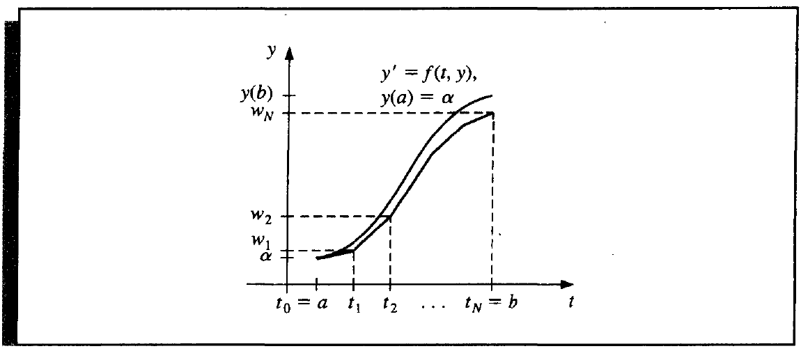
General Idea¶

Of all the method we introduce below, we can only approximate some points, but not the whole function $y(t)$. The approximation points are called mesh points. Moreover, we will only approximate the equally spaced points. Suppose we apporximate the values at $N$ points on $[a, b]$, then the mesh points are

\[ t_i = a + ih, \]

where $h = (b - a) / N$ is the step size. To get the value between mesh points, we can use interpolation method. Since we know the derivative value $f(t, y)$ at the mesh point, it's nice to use Hermit interpolation or cubic spline interpolation.

Availability and Uniqueness¶

Before finding out the approximation, we need some conditions to guarantee its availability and uniqueness.

Definition 5.0

$f(t, y)$ is said to satisfy a Lipschitz condition in the variable $y$ on a set $D \in \mathbb{R}^2$ if $\exists\ L > 0$, s.t.

\[ |f(t, y_1) - f(t, y_2)| \le L|y_1 - y_2|,\ \ \forall\ (t, y_1), (t, y_2) \in D. \]

$L$ is called a Lipschitz constant for $f$.

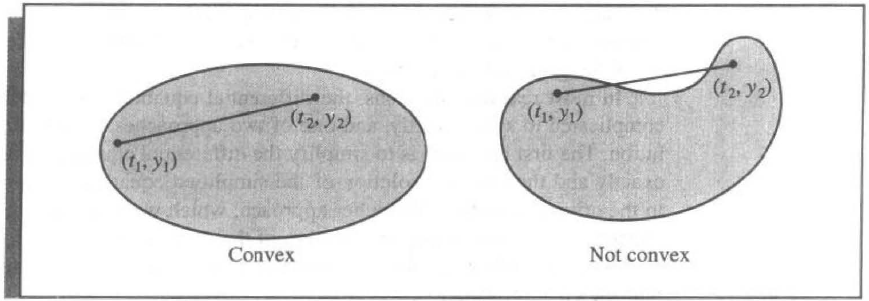
Definition 5.1

A set $D \in \mathbb{R}^2$ is said to be convex if

\[ \forall\ (t, y_1), (t, y_2) \in D,\ \ \forall\ \lambda \in [0, 1],\ \ ((1 - \lambda)t_1 + \lambda t_2, (1 - \lambda)y_1 + \lambda y_2) \in D. \]

Theorem 5.0 | Sufficient Condition

$f(t, y)$ is defined on a convex set $D \in \mathbb{R}^2$. If $\exists\ L > 0$ s.t.

\[ \left|\frac{\partial f}{\partial y}(t, y)\right| \le L,\ \ \forall\ (t, y) \in D, \]

then $f$ satisfies a Lipschitz condition on $D$ in the variable $y$ with Lipschitz constatnt $L$.

Theorem 5.1 | Unique Solution

$f(t, y)$ is continuous on $D = \{(t, y) | a \le t \le b, -\infty < y < \infty\}$($D$ is convex). If $f$ satisfies a Lipschitz condition on $D$ in the variable $y$, then the IVP

\[ y'(t) = f(t, y),\ \ a \le t \le b,\ \ y(a) = \alpha, \]

has a unique solution $y(t)$ for $a \le t \le b$.

Definition 5.2

The IVP

\[ \frac{dy}{dt} = f(t, y),\ a \le t \le b,\ y(a) = \alpha, \]

is said to be a well-posed problem if

A unique solution $y(t)$ exists;
$\forall\ \varepsilon > 0, \exists\ k(\varepsilon) > 0$, s.t. $\forall |\varepsilon_0| < \varepsilon$, and $|\delta(t)|$ is continuous with $|\delta(t)| < \varepsilon$ on $[a, b]$, a unique solution $z(t)$ to the IVP

\[ \frac{dz}{dt} = f(t, y) + \delta(t),\ \ a \le t \le b,\ \ y(a) = \alpha,\ \ \text{ (perturbed problem)} \]

exists with

\[ |z(t) - y(t)| < k(\varepsilon)\varepsilon,\ \ \forall\ t \in [a, b]. \]

Numerical methods will always be concerned with solving a perturbed problem since roundoff error is unavoidable. Thus we want the problem to be well-posed, which means the perturbation will not affect the result approxiamtion a lot.

Theorem 5.2

$f(t, y)$ is continuous on $D = \{(t, y) | a \le t \le b, -\infty < y < \infty\}$($D$ is convex). If $f$ satisfies a Lipschitz condition on $D$ in the variable $y$, then the IVP

\[ y'(t) = f(t, y),\ \ a \le t \le b,\ \ y(a) = \alpha, \]

is well-posed.

Besides, we also need to discuss the sufficient condition of mth-order system of first-order IVP.

Similarly, we have the definition of Lipschitz condition and it's sufficient for the uniqueness of the solution.

Definition 5.3

$f(t, y_1, \dots, y_m)$ define on the convex set

\[ D = \{(t, y_1, \dots, y_m | a \le t \le b, -\infty < u_i < \infty, \text{ for each } i = 1, 2, \dots, m\} \]

is said to satisfy Lipschitz condition on $D$ in the variables $y_1, \dots, y_m$ if $\exists\ L > 0$, s.t

\[ \begin{aligned} & \forall\ (t, y_1, \dots, y_n), (t, z_1, \dots, z_n) \in D, \\ & |f(t, y_1, \dots, y_m) - f(t, z_1, \dots, z_m)| \le L \sum\limits_{j = 1}^m |y_j - z_j|. \end{aligned} \]

Theorem 5.3

if $f(t, y_1, \dots, y_m)$ satisfy Lipschitz condition, then the mth order systems of first-order IVP has a unique solution $y_1(t), \dots, y_n(t)$.

Euler's Method¶

To measure the error of Taylor methods (Euler's method is Taylor's method of order 1), we first give the definition of local truncation error, which somehow measure the truncation error at a specified step.

Definition 5.4

The difference method

\[ \begin{aligned} w_0 &= \alpha, \\ w_{i + 1} &= w_i + h\phi(t_i, w_i). \end{aligned} \]

has the local truncation error

\[ \tau_{i + 1}(h) = \frac{y_{i + 1} - (y_i + h\phi(t_i, y_i))}{h} = \frac{y_{i + 1} - y_i}{h} - \phi(t_i, y_i). \]

Forward / Explicit Euler's Method¶

We use Taylor's Theorem to derive Euler's method. Suppose $y(t)$ is the unique solution of IVP, for each mesh points, we have

\[ y(t_{i + 1}) = y(t_i) + hy'(t_i) + \frac{h^2}{2}y''(\xi_i), \xi_i \in [t_i, t_{i + 1}], \]

and since $y'(t_i) = f(t_i, y(t_i))$, we have

\[ y(t_{i + 1}) = y(t_i) + hf.(t_i, y(t_i)) + \frac{h^2}{2}y''(\xi_i), \xi_i \in [t_i, t_{i + 1}]. \]

If $w_i \approx y(t_i)$ and we delete the remainder term, we get the (Explicit) Euler's method.

(Explicit) Euler's Method

\[ \begin{aligned} w_0 &= \alpha, \\ w_{i + 1} &= w_i + hf(t_i, w_i). \text{(difference equations)} \end{aligned} \]

The local truncation error of Euler's Method is

\[ \tau_{i + 1}(h) = \frac{hy'(t_i) + \frac{h^2}{2}y''(\xi_i)}{h} - f(t_i, y_i) = \frac{h}{2}y''(\xi_i) = O(h). \]

Theorem 5.4

The error bound of Euler's method is

\[ |y(t_i) - w_i| \le \frac{hM}{2L}\left[e^{L(t_i - a)} - 1\right], \]

where $M$ is the upper bound of $|y''(t)|$.

Although it has an exponential term (which is not such an accurate error bound), the most important intuitive is that the error bound is proportional to $h$.

If we consider the roundoff error, we have the following theorem.

Theorem 5.5

Suppose there exists roundoff error and $u_i = w_i + \delta_i$, $i = 0, 1, \dots$, then

\[ |y(t_i) - u_i| \le \frac{1}{L}\left(\frac{hM}{2} + \frac{\delta}{h}\right)\left[e^{L(t_i - a)} - 1\right] + |\delta_0|e^{L(t_i - a)}, \]

where $\delta$ is the upper bound of $\delta_i$.

This comes to a different case, we can't make $h$ too small, and the optimal choice of $h$ is

\[ h = \sqrt{\frac{2\delta}{M}}. \]

Backward/ Implicit Euler's Method¶

Inversely, if we use Taylor's Theorem in the following way,

\[ y(t_i) = y(t_{i + 1}) - hy'(t_{i + 1}) + \frac{h^2}{2}y''(\xi_{i + 1}), \xi_i \in [t_i, t_{i + 1}]. \]

Thus we get the Implicit Euler's Method,

Implicit Euler's Method

\[ \begin{aligned} w_0 &= \alpha, \\ w_{i + 1} &= w_i + hf(t_{i + 1}, w_{i + 1}). \end{aligned} \]

Since $w_{i + 1}$ is on the both side, we may use some methods in Chapter 2 to solve out the equation.

The local truncation error of implicit Euler's method is

\[ \begin{aligned} \tau_{i + 1}(h) &= \frac{hy'(t_i) + \frac{h^2}{2}y''(\xi_i)}{h} - f(t_{i + 1}, y_{i + 1}) \\ &= y'(t_i) - y'(t_{i + 1}) + \frac{h}{2}y''(\xi_i) \\ &= y'(t_i) - y'(t_i) - hy''(\xi'_i) + \frac{h}{2}y''(\xi_i) \\ &= -\frac{h}{2}y''(\eta_i) = O(h). \end{aligned} \]

Trapezoidal Method¶

Notice the local truncation errors of two Euler's method are

\[ \tau_{i + 1}(h) = \frac{h}{2}y''(\xi'),\ \ \tau_{i + 1}(h) = -\frac{h}{2}y''(\eta'). \]

If we combine these two, we then obtain a method of $O(h^2)$ local truncation error, which is called Trapezoidal Method.

Trapezoidal Method

\[ \begin{aligned} w_0 &= \alpha, \\ w_{i + 1} &= w_i + \frac{h}{2}[f(t_i, w_i) + f(t_{i + 1}, w_{i + 1})]. \end{aligned} \]

Higher-Order Taylor Method¶

In Euler's methods, we only employ first order Taylor polynomials. If we expand it more to nth Taylor polynomials, we have

\[ \begin{aligned} y(t_{i + 1}) &= y(t_i) + hy'(t_i) + \frac{h^2}{2}y''(t_i) + \cdots + \frac{h^n}{n!}y^{(n)}(t_i) + \frac{h^{n + 1}}{(n + 1)!} y^{(n + 1)}(\xi_i), \\ & \text{ where } \xi_i \in [t_i, t_{i + 1}], \end{aligned} \]

and since $y^{(k)}(t) = f^{(k - 1)}(t, y(t))$, we have

\[ \begin{aligned} y(t_{i + 1}) &= y(t_i) + hf(t_i, y(t_i)) + \frac{h^2}{2}f'(t_i, y(t_i)) + \cdots + \frac{h^n}{n!}f^{(n - 1)}(t_i, y(t_i)) \\ & \ \ \ \ + \frac{h^{n + 1}}{(n + 1)!} f^{(n)}(\xi_i, y(\xi_i)). \end{aligned} \]

Taylor Method of order n

\[ \begin{aligned} w_0 &= \alpha, \\ w_{i + 1} &= w_i + hT^{(n)}(t_i, w_i), \end{aligned} \]

where

\[ T^{(n)}(t_i, w_i) = f(t_i, w_i) + \frac{h}{2}f'(t_i, w_i) + \cdots + \frac{h^{n - 1}}{n!}f^{(n - 1)}(t_i, w_i). \]

Theorem 5.6

The local truncation error of Taylor method of order $n$ is $O(h^n)$.

Runge-Kutta Method¶

Although Taylor method gives more accuracy as $n$ increase, but it's not an easy job to calculate nth derivative of $f$. Here we introduce a new method called Runge-Kutta Method, which has low local truncation error and doesn't need to compute derivatives. It's based on Taylor's Theorem in two variables.

Theorem 5.7 | Taylor's Theorem in two variables (Recap)

$f(x, y)$ has continous $n + 1$ partial derivatives on the neigbourhood of $A(x_0, y_0)$, denoted by $U(A)$, then $\forall\ (x, y) \in U(A)$, denote $\Delta x = x - x_0$, $\Delta y = y - y_0$, $\exists\ \theta \in (0, 1)$, s.t.

\[ f(x, y) = P_n(x, y) + R_n(x, y), \]

where

\[ \small \begin{aligned} P_n(x, y) &= f(x_0, y_0) + \left(\Delta x\frac{\partial}{\partial x} + \Delta y \frac{\partial}{\partial y}\right)f(x_0, y_0) + \frac{1}{2!}\left(\Delta x\frac{\partial}{\partial x} + \Delta y \frac{\partial}{\partial y}\right)^2f(x_0, y_0) + \\ & \ \ \ \ \ \cdots + \frac{1}{n!}\left(\Delta x\frac{\partial}{\partial x} + \Delta y \frac{\partial}{\partial y}\right)^nf(x_0, y_0), \end{aligned} \]

\[ \small R_n(x, y) = \frac{1}{(n + 1)!}\left(\Delta x\frac{\partial}{\partial x} + \Delta y \frac{\partial}{\partial y}\right)^{n + 1}f(x_0 + \theta \Delta x, y_0 + \theta \Delta y). \]

and

\[ \small \left(\Delta x\frac{\partial}{\partial x} + \Delta y \frac{\partial}{\partial y}\right)^{k}f(x, y) = \sum\limits_{i = 0}^k \binom{k}{i} (\Delta x)^i (\Delta y)^{k - i} \frac{\partial^k f}{\partial x^i \partial y^{k - i}}(x, y). \]

Derivation of Midpoint Method

To equate

\[ T^{(2)}(t, y) = f(t, y) + \frac{h}{2}f'(t, y) = f(t, y) + \frac{h}{2}\frac{\partial f}{\partial t}(t,y) + \frac{h}{2}\frac{\partial f}{\partial y}(t,y)\cdot f(t, y), \]

with

\[ \begin{aligned} a_1f(t + \alpha_1, y + \beta_1) &= a_1f(t, y) + a_1 \alpha_1 \frac{\partial f}{\partial t}(t, y) \\ & \ \ \ \ + a_1 \beta_1 \frac{\partial f}{\partial y}(t, y) + a_1 \cdot R_1(t + \alpha_1, y + \beta_1), \end{aligned} \]

except for the last residual term $R_1$, we have

\[ a_1 = 1,\ \ \alpha_1 = \frac{h}{2},\ \ beta_1 = \frac{h}{2}f(t, y). \]

Thus

\[ T^{(2)}(t, y) = f\left(t + \frac{h}{2}, y + \frac{h}{2}f(t, y)\right) - R_1. \]

Since the term $R_1$ is only concerned with the 2^nd-order partial derivatives of $f$, if they are bounded, then $R_1$ is $O(h^2)$, the order of the local truncation error. Replace $T^{(2)}(t,y)$ by the formula above in the Taylor method of order 2, we have the Midpoint Method.

Midpoint Method

\[ \begin{aligned} w_0 &= \alpha, \\ w_{i + 1} &= w_i + hf\left(t_i + \frac{h}{2}, w_i + \frac{h}{2}f(t_i, w_i)\right). \end{aligned} \]

Derivation of Modified Euler Method and Heun's Method

Similarly, approximate

\[ T^{(3)}(t, y) = f(t, y) + \frac{h}{2}f'(t, y) + \frac{h^2}{6}f''(t,y), \]

with

\[ a_1f(t,y) + a_2f(t + \alpha_2, y + \delta_2f(t,y)). \]

But it doesn't have sufficient equation to determine the 4 unknowns $a_1, a_2, \alpha_2, \delta_2$ above. Instead we have

\[ a_1 + a_2 = 1, \ \alpha_2 = \delta_2\ \overset{\Delta}{=\!=}\ ph. \]

Thus a number of $O(h^2)$ methods can be derived, and they are generally in the form

\[ \begin{aligned} w_{i + 1} &= w_i + h(a_1 K_1 + a_2 K_2) \\ K_1 &= f(t_i, w_i), \\ K_2 &= f(t_i + ph, y + ph K_1). \end{aligned} \]

The most important are the following two.

Modified Euler Method

\[ \begin{aligned} w_0 &= \alpha, \\ w_{i + 1} &= w_i + \frac{h}{2}[f(t_i, w_i) + f(t_i + h, w_i + hf(t_i, w_i))]. \end{aligned} \]

Heun's Method

\[ \begin{aligned} w_0 &= \alpha, \\ w_{i + 1} &= w_i + \frac{h}{4}\left[f(t_i, w_i) + 3f\left(t_i + \frac23 h, w_i + \frac23 hf(t_i, w_i)\right)\right]. \end{aligned} \]

In a similar manner, approximate $T^{(n)}(t, y)$ with

\[ \lambda_1 K_1 + \lambda_2 K_2 + \cdots + \lambda_m K_m, \]

where

\[ \begin{aligned} K_1 &= f(t, y), \\ K_2 &= f(t + \alpha_2 h, y + \beta_{21} h K_1), \\ & \ \ \vdots \\ K_m &= f(t + \alpha_m h, y + \beta_{m1} h K_1 + \beta_{m, m - 1} hK_{m - 1}), \end{aligned} \]

with different $m$, we can derive quite a lot of Runge-Kutta methods.

The most common Runge-Kutta method is given below.

Runge-Kutta Order Four

\[ \begin{aligned} w_0 &= \alpha, \\ w_{i + 1} &= w_i + \frac{h}{6}(K_1 + 2K_2 + 2K_3 + K_4), \\ K_1 &= f(t_i, w_i), \\ K_2 &= f\left(t_i + \frac{h}{2}, w_i + \frac{h}{2}K_1\right), \\ K_3 &= f\left(t_i + \frac{h}{2}, w_i + \frac{h}{2}K_2\right), \\ K_4 &= f\left(t_i + h, w_i + h K_3\right). \end{aligned} \]

The local trancation error of Runge-Kutta are given below, where $n$ is the number of evaluations per step.

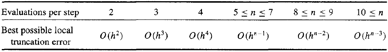
Property

Compared to Taylor's method, evaluate $f(t, y)$ the same times, Runge-Kutta gives the lowest error.

Multistep Method¶

In the previous section, the difference equation only relates $w_{i + 1}$ with $w_{i}$. Multistep Method discuss the situation of relating more term of previous predicted $w$.

Definition 5.5

An m-step multistep method for solving the IVP

\[ y'(t) = f(t, y),\ \ a \le t \le b,\ \ y(a) = \alpha, \]

has a difference equation

\[ \begin{aligned} w_{i + 1} &= a_{m - 1}w_i + a_{m - 2}w_{i - 1} + \cdots a_0 w_{i + 1 - m} + h[b_mf(t_{i + 1}, w_{i + 1}) \\ & \ \ \ \ + b_{m - 1}f(t_i, w_i) + \cdots + b_0 f(t_{i + 1 - m}, w_{i + 1 - m})], \end{aligned} \]

with the starting values

\[ w_0 = \alpha,\ \ w_1 = \alpha_1,\ \ \dots,\ \ w_{m - 1} = \alpha_{m - 1}. \]

If $b_m = 0$, it's called explicit, or open. Otherwise, it's called implicit, or closed.

Similarly, we first define local truncation error for multistep method to measure the error at a specified step.

Definition 5.6

For a m-step multistep method, the local truncation error at $(i + 1)$th step is

\[ \begin{aligned} \tau_{i + 1}(h) &= \frac{y(t_{i + 1}) - a_{m - 1}y(t_i) - \cdots - a_0 y(t_{i + 1 - m})}{h} \\ & \ \ \ \ - b_{m - 1}f(t_i, y(t_{i + 1})) + \cdots + b_0 f(t_{i + 1 - m}, y(t_{i + 1 - m}))]. \end{aligned} \]

Adams Method¶

In this section, we only consider the case of $a_{m - 1} = 1$ and $a_i = 0$, $i \ne m - 1$.

To derive the Adams method, we start from a simple formula.

\[ y(t_{i + 1}) - y(t_i) = \int_{t_i}^{t_{i + 1}}y'(t)dt = \int_{t_i}^{t_{i + 1}}f(t, y(t))dt. \]

i.e.

\[ y(t_{i + 1}) = y(t_i) + \int_{t_i}^{t_{i + 1}}f(t, y(t))dt. \]

We cannot integrate $f(t, y(t))$ without knowing $y(t)$. Instead we use an interpolating polynomial $P(t)$ by points $(t_0, w_0),\ \dots,\ (t_i, w_i)$ to approximate $f(t, y)$. Thus we approximate $y(t_{i + 1})$ by

\[ y(t_{i + 1}) \approx w_i + \int_{t_i}^{t_{i + 1}} P(t) dt. \]

For convenience, we use Newton backward-difference formula to represent $P(t)$.

Adams-Bashforth m-Step Explicit Method¶

To derive an Adam-Bashforth explicit m-step technique, we form the interpolating polynomial $P_{m - 1}(t)$ by

\[ (t_i, f(t_i, y(t_i))),\ \ \dots,\ \ (t_{i + 1 - m}, f(t_{i + 1 - m}, y(t_{i + 1 - m}))). \]

Then suppose $t = t_i + sh$, with $dt = hds$, we have

\[ \begin{aligned} \int_{t_i}^{t_{i + 1}} f(t, y(t)) dt &= \int_{t_i}^{t_{i + 1}} \sum\limits_{k = 0}^{m - 1}(-1)^k \binom{-s}{k}\nabla^k f(t_i, y(t_i))dt \\ & \ \ \ \ + \int_{t_i}^{t_{i + 1}} \frac{f^{(m)}(\xi_i, y(\xi_i))}{m!}\prod\limits_{k = 0}^{m - 1}(t - t_{i - k})dt \\ \left(\text{Note that } dt = hds\right) &= h\sum\limits_{k = 0}^{m - 1}\nabla^k (-1)^k \int_0^1 \binom{-s}{k}ds \\ & \ \ \ \ + h^{m + 1}\int_0^1 \binom{-s}{m}f^{(m)}(\xi_i, y(\xi_i))ds. \\ \left(\substack{\text{Weighted Mean Value} \\ \text{Theorem for Integral}}\right) &= h\sum\limits_{k = 0}^{m - 1}\nabla^k (-1)^k \int_0^1 \binom{-s}{k}ds \\ & \ \ \ \ + h^{m + 1}f^{(m)}(\mu_i, y(\mu_i))\int_0^1 \binom{-s}{m}ds. \end{aligned} \]

Since for a given $k$, we have

$k$	$0$	$1$	$2$	$3$	$4$
$(-1)^k\int_0^1 \binom{-s}{k}ds$	$1$	$\frac12$	$\frac{5}{12}$	$\frac38$	$\frac{251}{720}$

Thus

\[ \begin{aligned} y(t_{i + 1}) &= y(t_i) + h\left[f(t_i, y(t_i)) + \frac12 \nabla f(t_i, y(t_i)) + \frac{5}{12} \nabla^2 f(t_i, y(t_i)) + \cdots\right] \\ & \ \ \ \ + h^{m + 1}f^{(m)}(\mu_i, y(\mu_i))\int_0^1 \binom{-s}{m}ds. \end{aligned} \]

Adams-Bashforth m-Step Explicit Method

\[ w_0 = \alpha,\ \ w_1 = \alpha_1,\ \ \dots,\ \ w_{m - 1} = \alpha_{m - 1}, \]

\[ w_{i + 1} = w_i + h\sum\limits_{k = 0}^{m - 1}\nabla^k f(t_i, y(t_i)) (-1)^k \int_0^1 \binom{-s}{k}ds, \]

with local truncation error

\[ \tau_{i + 1}(h) = h^{m}y^{(m + 1)}(\mu_i)(-1)^m\int_0^1 \binom{-s}{m}ds. \]

Adams-Bashforth Two-Step Explicit Method

\[ w_0 = \alpha,\ \ w_1 = \alpha_1, \]

\[ w_{i + 1} = w_i + \frac{h}{2}[3f(t_i, w_i) - f(t_{i - 1}, w_{i - 1})], \]

with local truncation error

\[ \tau_{i + 1}(h) = \frac{5}{12}y'''(\mu_i)h^2. \]

Adams-Bashforth Three-Step Explicit Method

\[ w_0 = \alpha,\ \ w_1 = \alpha_1,\ \ w_2 = \alpha_2, \]

\[ w_{i + 1} = w_i + \frac{h}{12}[23f(t_i, w_i) - 16f(t_{i - 1}, w_{i - 1}) + 5f(t_{i - 2}, w_{i - 2})], \]

with local truncation error

\[ \tau_{i + 1}(h) = \frac{3}{8}y^{(4)}(\mu_i)h^3. \]

Adams-Bashforth Four-Step Explicit Method

\[ w_0 = \alpha,\ \ w_1 = \alpha_1,\ \ w_2 = \alpha_2,\ \ w_3 = \alpha_3, \]

\[ \begin{aligned} w_{i + 1} = w_i + \frac{h}{24}&[55f(t_i, w_i) - 59f(t_{i - 1}, w_{i - 1}) \\ & + 37f(t_{i - 2}, w_{i - 2}) - 9f(t_{i - 3}, w_{i - 3})], \end{aligned} \]

with local truncation error

\[ \tau_{i + 1}(h) = \frac{251}{720}y^{(5)}(\mu_i)h^4. \]

Adams-Moulton m-Step Implicit Method¶

For implicit case, we add $(t_{i + 1}, f(t_{i + 1}, y(t_{i + 1})))$ as one more interpolating node to construct the interpolating polynomials. Let $t = t_{i + 1} + sh$ and there is $m$ points. Similarly we have the conclusions below.

Adams-Moulton m-Step Implicit Method

\[ w_0 = \alpha,\ \ w_1 = \alpha_1,\ \ \dots,\ \ w_{m - 1} = \alpha_{m - 1}, \]

\[ w_{i + 1} = w_i + h\sum\limits_{k = 0}^{m}\nabla^k f(t_{i + 1}, y(t_{i + 1})) (-1)^k \int_{-1}^0 \binom{-s}{k}ds, \]

with local truncation error

\[ \tau_{i + 1}(h) = h^{m + 1}y^{(m + 2)}(\mu_i)(-1)^{m + 1}\int_{-1}^0 \binom{-s}{m + 1}ds. \]

Adams-Moulton Two-Step Implicit Method

\[ w_0 = \alpha,\ \ w_1 = \alpha_1, \]

\[ w_{i + 1} = w_i + \frac{h}{12}[5f(t_{i + 1}, w_{i + 1}) + 8f(t_i, w_i) - f(t_{i - 1}, w_{i - 1})], \]

with local truncation error

\[ \tau_{i + 1}(h) = -\frac{1}{24}y^{(4)}(\mu_i)h^3. \]

Adams-Moulton Three-Step Implicit Method

\[ w_0 = \alpha,\ \ w_1 = \alpha_1,\ \ w_2 = \alpha_2, \]

\[ w_{i + 1} = w_i + \frac{h}{24}[9f(t_{i + 1}, w_{i + 1}) + 19f(t_i, w_i) - 5f(t_{i - 1}, w_{i - 1}) + f(t_{i - 2}, w_{i - 2})], \]

with local truncation error

\[ \tau_{i + 1}(h) = -\frac{19}{720}y^{(5)}(\mu_i)h^4. \]

Adams-Moulton Four-Step Implicit Method

\[ w_0 = \alpha,\ \ w_1 = \alpha_1,\ \ w_2 = \alpha_2,\ \ w_3 = \alpha_3, \]

\[ \begin{aligned} w_{i + 1} = w_i + \frac{h}{720}&[251f(t_{i + 1}, w_{i + 1}) + 646f(t_i, w_i) - 264f(t_{i - 1}, w_{i - 1}) \\ & + 106f(t_{i - 2}, w_{i - 2}) - 19f(t_{i - 3}, w_{i - 3})], \end{aligned} \]

with local truncation error

\[ \tau_{i + 1}(h) = -\frac{3}{160}y^{(6)}(\mu_i)h^5. \]

Note

Comparing an m-step Adams-Bashforth explicit method and (m - 1)-step Adams-Moulton implicit method, they both involve m evaluation of $f$ per step, and both have the local truncation error of the term $ky^{(m + 1)}(\mu_i)h^m$. And the latter implicit method has the smaller coefficient $k$. This leads to greater stability and smaller roundoff errors for implicit methods.

Predictor-Corrector Method¶

Implicit method has some advantages but it's hard to calculate. We could use some iterative methods introduced in Chapter 2 to solve it but it complicates the process considerably.

In practice, since explicit method is easy to calculate, we combine the explicit and implicit method to predictor-corrector method.

Predictor-Corrector Method

Step.1 Compute first $m$ initial values by Runge-Kutta method.

Step.2 Predict by Adams-Bashforth explicit method.

Step.3 Correct by Adams-Moulton implicit method.

NOTE: All the formulae used in the three steps have the same order of truncation error.

Example

Take $m = 4$ which is the most common case as exmaple.

Step.1

From initial value $w_0 = \alpha$, we use Runge-Kutta method of order four to derive $w_1$, $w_2$ and $w_3$. Set $i = 3$.

Step.2

Use four-step Adams-Bashforth explicit method, we have

\[ \small w_{i + 1}^{(0)} = w_i + \frac{h}{24}[55f(t_i, w_i) - 59f(t_{i - 1}, w_{i - 1}) + 37f(t_{i - 2}, w_{i - 2}) - 9f(t_{i - 3}, w_{i - 3})], \]

Step.3

Use three-step Adams-Moulton

\[ \small w_{i + 1}^{(1)} = w_i + \frac{h}{24}[9f(t_{i + 1}, w_{i + 1}^{(1)}) + 19f(t_i, w_i) - 5f(t_{i - 1}, w_{i - 1}) + f(t_{i - 2}, w_{i - 2})], \]

Then we have two options

$i = i + 1$, and go back to Step. 2, to approximate the next point.
Or, for higher accuracy, we can repeat Step.3 iteratively by

\[ \small w_{i + 1}^{(k + 1)} = w_i + \frac{h}{24}[9f(t_{i + 1}, w_{i + 1}^{(k)}) + 19f(t_i, w_i) - 5f(t_{i - 1}, w_{i - 1}) + f(t_{i - 2}, w_{i - 2})]. \]

Other Methods¶

If we derive the multistep method by Taylor expansion, we can have more methods. We take an example to show it.

Suppose we want to derive a difference equation in the form

\[ w_{i + 1} = a_0 w_{i - 1} + h(b_2 f(t_{i + 1}, w_{i + 1}) + b_1 f(t_i, w_i) + b_0 f(t_{i - 1}, w_{i - 1})). \]

We use $y_i$ and $f_i$ to denote $y(t_i)$ and $f(t_i, y_i)$ respectively.

Expand $y_{i - 1}, f_{i + 1}, f_{i}, f_{i - 1}$, we have

\[ \begin{aligned} y_{i - 1} &= y_i - hy_i' + \frac12 h^2 y_i'' - \frac16h^3y_i''' + O(h^4), \\ f_{i + 1} &= y_i' + hy_i'' + \frac12 h^2 y_i''' + O(h^3), \\ f_i &= y_i', \\ f_{i - 1} &= y_i' - hy_i'' + \frac12 h^2 y_i''' + O(h^3), \\ \end{aligned} \]

and note that

\[ y_{i + 1} = y_i + hy_i' + \frac12 h^2 y_i'' + \frac16 h^3 y_i'''+ O(h^4). \]

Equate them with

\[ y_{i + 1} = a_0 y_{i - 1} + h(b_2 f_{i + 1} + b_1 f_i + b_0 f_{i - 1}). \]

We can solve out

\[ a_0 = 1,\ \ b_2 = \frac13,\ \ b_1 = \frac43,\ \ b_0 = \frac13. \]

Thus

\[ w_{i + 1} = w_{i - 1} + \frac{h}{3}(f(t_{i + 1}, w_{i + 1}) + 4f(t_i, w_i) + f(t_{i - 1}, w_{i - 1})). \]

Simpson Implicit Method

\[ w_0 = \alpha,\ \ w_1 = \alpha_1, \\ w_{i + 1} = w_{i - 1} + \frac{h}{3}(f(t_{i + 1}, w_{i + 1}) + 4f(t_i, w_i) + f(t_{i - 1}, w_{i - 1})), \]

with local truncation error

\[ \tau_{i + 1}(h) = \frac{h^4}{90}y^{(5)}(\xi_i). \]

Note that it's an implicit method, and the most commonly used corresponding predictor is

Milne's Method

\[ w_0 = \alpha,\ \ w_1 = \alpha_1,\ \ w_2 = \alpha_2 \\ w_{i + 1} = w_{i - 3} + \frac{4h}{3}(2f(t_i, w_i) + - f(t_{i - 1}, w_{i - 1}) + 2f(t_{i - 2}, w_{i - 2})), \]

with local truncation error

\[ \tau_{i + 1}(h) = \frac{14}{90}h^4 y^{(5)}(\xi_i). \]

which can also derive by Taylor expansion in the similar manner.

Higher-Order Systems of First-Order IVP¶

Actually it just vectorize the method that we've mentioned above. Take Runge-Kutta Order Four as example.

Runge-Kutta Method for Systems of Differential Equations

\[ \begin{aligned} w_{1, 0} &= \alpha_1, w_{2, 0} = \alpha_2, \dots, w_{m, 0} = \alpha_m. \\ w_{i, j + 1} &= w_{i, j} + \frac{h}{6}(K_{1, i} + 2K_{2, i} + 2K_{3, i} + K_{4, i}), \\ K_{1, i} &= f_i(t_j, w_{1, j}, w_{2, j}, \dots, w_{m, j}), \\ K_{2, i} &= f_i\left(t_j + \frac{h}{2}, w_{1, j} + \frac{h}{2}K_{1, 1}, w_{2, j} + \frac{h}{2}K_{1, 2}, \dots, w_{m, j} + \frac{h}{2}K_{1, m}\right), \\ K_{3, i} &= f_i\left(t_j + \frac{h}{2}, w_{1, j} + \frac{h}{2}K_{2, 1}, w_{2, j} + \frac{h}{2}K_{2, 2}, \dots, w_{m, j} + \frac{h}{2}K_{2, m}\right), \\ K_{4, i} &= f_i\left(t_j + h, w_{1, j} + h K_{3, 1}, w_{2, j} + h K_{3, 2}, \dots, w_{m, j} + h K_{3. m} \right). \end{aligned} \]

Higher-Order IVP¶

We can deal with higher-order IVP the same as higher-order systems of first-order IVP. The only transformation we need to do is to let $u_1(t) = y(t)$, $u_2(t) = y'(t)$, $\dots$, and $u_m(t) = y^{(m - 1)}(t)$.

This produces the first-order system

\[ \begin{aligned} \frac{du_1}{dt} &= \frac{dy}{dt} = u_2, \\ \frac{du_2}{dt} &= \frac{dy'}{dt} = u_3, \\ & \vdots \\ \frac{du_{m - 1}}{dt} &= \frac{dy^{(m - 2)}}{dt} = u_m, \\ \frac{du_m}{dt} &= \frac{dy^{(m - 1)}}{dt} = y^{(m)} = f(t, y', y'', \dots, y^{(m - 1)}) = f(t, u_1, \dots, u_m), \end{aligned} \]

with initial conditions

\[ u_1(a) = y(a) = \alpha_1,\ \ u_2(a) = y'(a) = \alpha_2,\ \ \dots,\ \ u_m(a) = y^{(m - 1)}(a) = \alpha_m. \]

Stability¶

Definition 5.7

A one-step difference-equation method with local truncation error $\tau_i(h)$ is consistent with the differential equation it approximates if

\[ \lim\limits_{h \rightarrow 0} \max\limits_{1 \le i \le N}|\tau_i(h)| = 0. \]

For m-step multistep methods, it's also required that

\[ \lim\limits_{h \rightarrow 0} |\alpha_i - y_i| = 0,\ \ i = 1, 2, \dots, m - 1, \]

since at most cases, these $\alpha_i$ are derived by one-step methods.

Definition 5.8

A one-step / multistep difference-equation method is convergent w.r.t the differential equation it approximates if

\[ \lim\limits_{h \rightarrow 0} \max\limits_{1 \le i \le N}|w_i - y(t_i)| = 0. \]

Definition 5.9

A stable method is one whose results depent continously on the initial data, in the sense that small changes or perturbations in the intial conditions produce correspondingly small changes in the subsequent approximations.

One Step Method¶

It's relatively natural to think the stability is somewhat analogous to the discussion of well-posed, and thus it's not surprising Lipschitz condition appears. The following theorem gives the relation among consistency, convergence and stability.

Theorem 5.8

Suppose the IVP is approximated by a one-step method in the form

\[ \begin{aligned} w_0 &= \alpha, \\ w_{i + 1} &= w_i + h \phi(t_i, w_i, h). \end{aligned} \]

If $\exists\ h_0 > 0$ and $ \phi(t, w, h)$ is continuous and satisfies a Lipschitz condition in the varaible $w$ with Lipschitz constant $L$ on the set

\[ D = \{(t, w, h) | a \le t \le b, -\infty < w < \infty, 0 \le h \le h_0\}. \]

Then

The method is stable.
The difference method is convergent iff it's consistent, which is equivalent to

\[ \phi(t, y, 0) = f(t, y),\ \ t \in [a, b]. \]

(Relation between Global Error and Local Truncation Error) If $\exists \tau(h)$ s.t. $|\tau_i(h)| \le \tau(h)$ whenever $0 \le h \le h_0$, then

\[ |y(t_i) - w_i| \le \frac{\tau(h)}{L}e^{L(t_i - a)}. \]

Multistep Method¶

Theorem 5.9 | Relation between Global Error and Local Truncation Error

Suppose the IVP is approximated by a predictor-corrector method with an m-step Adams-Bashforth predictor equation

\[ w_{i + 1} = w_i + h[b_{m - 1}f(t_i, w_i) + \cdots + b_0f(t_{i + 1 - m}, w_{i + 1 - m})], \]

with local truncation error $\tau_{i + 1}(h)$, and an (m - 1)-step Adams-Moulton corrector eqation

\[ w_{i + 1} = w_i + h[\tilde b_{m - 1}f(t_i, w_i) + \cdots + \tilde b_0f(t_{i + 1 - m}, w_{i + 1 - m})], \]

with local truncation error $\tilde \tau_{i + 1}(h)$. In addition, suppose $f(t, y)$ and $f_y(t, y)$ are continous on $D = \{(t, y) | a \le t \le b, -\infty < y < \infty\}$ and $f_y$ is bounded. Then the local truncation error $\sigma_{i + 1}(h)$ of the predictor-corrector method is

\[ \small \sigma_{i + 1}(h) = \tilde \tau_{i + 1}(h) + \tau_{i + 1}(h) \tilde b_{m - 1} \frac{\partial f}{\partial y}(t_{i + 1}, \theta_{i + 1}),\ \ \text{ for some } \theta_{i + 1} \in (0, h\tau_{i + 1}(h)). \]

Moreover, $\exists\ k_1, k_2$, s.t.

\[ |w_i - y(t_i)| \le \left[\max\limits_{0 \le j \le m - 1}|w_j - y(t_j)| + k_1\sigma(h) \right] e^{k_2(t_i - a)}, \]

where $\sigma(h) = \max\limits_{m \le j \le N}|\sigma_j(h)|$.

For the difference equation of multistep method, we first introduce characteristc polynomial associated with the method, given by

\[ P(\lambda) = \lambda^m - a_{m - 1}\lambda^{m - 1} - a_{m - 2}\lambda^{m - 2} - \cdots - a_1 \lambda - a_0. \]

Definition 5.10

Suppose the roots of the characteristic equation

\[ P(\lambda) = \lambda^m - a_{m - 1}\lambda^{m - 1} - a_{m - 2}\lambda^{m - 2} - \cdots - a_1 \lambda - a_0 = 0 \]

associated with the multistep difference method

\[ w_0 = \alpha,\ \ w_1 = \alpha_1,\ \ \dots,\ \ w_{m - 1} = \alpha_{m - 1}, \\ w_{i + 1} = a_{m - 1}w_i + a_{m - 2}w_{i - 1} + \cdots a_0 w_{i + 1 - m} + hF(t_i, h, w_{i + 1}, w_i \dots, w_{i + 1 - m}). \]

If $|\lambda_i| \le 1$, for each $i = 1, 2, \dots, m$ and all roots with modulus value $1$ are simple roots, then the difference method is said to satisfy the root condition.

Methods that satisfy the root condition and have $\lambda = 1$ as the only root of the characteristic equation of magnitude one are called strongly stable.
Methods that satisfy the root condition and have more than one disctinct root with magnitude one are called weakly stable.
Methods that do not satisfy the root condition are called unstable.

Theorem 5.10

A multistep method of the form

\[ w_0 = \alpha,\ \ w_1 = \alpha_1,\ \ \dots,\ \ w_{m - 1} = \alpha_{m - 1}, \\ w_{i + 1} = a_{m - 1}w_i + a_{m - 2}w_{i - 1} + \cdots a_0 w_{i + 1 - m} + hF(t_i, h, w_{i + 1}, w_i \dots, w_{i + 1 - m}). \]

is stable iff it satisfies the root condition. Moreover, if the difference method is consistent with the differential equation, then the method is stable iff it is convergent.

Stiff Equations¶

However, a special type of solution is not easy to deal with, when the magnitude of derivative increases but the solution does not. They are call stiff equations.

Stiff differential eqaution are characterized as those whose exact solution has a term of the form $e^{-ct}$, where $c$ is a large positive constant. This is called the transient solution. Actaully there is another important part of solution called steady-state solution.

Let's first define test equation to examine what happen with the stiff cases.

Definition 5.11

A test equation is the IVP

\[ y' = \lambda y,\ \ y(0) = \alpha,\ \ \text{ where } \text{Re}(\lambda) < 0. \]

The solution is obviously $y(t) = \alpha e^{\lambda t}$, which is the transient solution. At this case, the steady-state solution is zero, thus the approximation characteristics of a method are easy to determine.

Example of Euler's Method

Take Euler's method as an example, and denote $H = h\lambda$. We have

\[ w_0 = \alpha, \\ w_{i + 1} = w_i + h(\lambda w_i) = (1 + h\lambda)w_i = (1 + H)w_i, \]

so

\[ w_{i + 1} = (1 + H)^{i + 1}w_0 = (1 + H)^{i + 1}\alpha. \]

The absolute error is

\[ |y(t_i) - w_i| = |(e^H)^i - (1 + H)^i||\alpha|. \]

When $H < 0$, $(e^H)^i$ decays to zero as $i$ increases. Thus we want $(1 + H)^i$ to decay too, which implies that

\[ |1 + H| < 1. \]

From another perspective, consider the roundoff error of the initial value $\alpha$ by,

\[ w_0 = \alpha + \delta_0. \]

At the ith step the roundoff error is

\[ \delta_i = (1 + H)^i \delta_0. \]

To control the error, we also want $|1 + H| < 1$.

In general, when applying to the test equation, we have the difference equation of the form

\[ w_{i + 1} = Q(H)w_i,\ \ H = h \lambda. \]

To make $Q(H)$ approximate $e^H$, we want at least $|Q(H)| < 1$ to make it decay to 0. The inequality delimit a region in a complex plane.

For a multistep method, the difference equation is in the form

\[ (1 - H b_m)w_{i + 1} - (a_{m - 1} + H b_{m - 1})w_i - \cdots - (a_0 + H b_0)w_{i + 1 - m} = 0. \]

We can define a characteristic polynomial

\[ Q(z, H) = (1 - H b_m)z^m - (a_{m - 1} + H b_{m - 1})z^{m - 1} - \cdots - (a_0 + H b_0). \]

Suppose $\beta_i$ are the distinct roots of $Q(z, H)$, then it can be proved that $\exists\ c_i$, s.t.

\[ w_{i} = \sum\limits_{k = 1}^m c_k\beta_k^i. \]

Again, to make $w_i$ approximate $(e^H)^i$, we want at least all $|\beta_k| < 1$ to make it decay to $0$. It also delimit a region in a complex plane.

Definition 5.12

The Region R of abosolute stability for a one-step method is

\[ R = \{H \in \mathbb{C} | |Q(H)| < 1\}, \]

and for a multistep method,

\[ R = \{H \in \mathbb{C} | |\beta_k| < 1,\ \ \text{ for all zero points of } Q(z, H)\}. \]

A numerical method is said to be A-stable if its region $R$ of abosolute stability contains left half-plane, which means $\text{Re}(\lambda) < 0$, stable with stiff equation.
Method A is said to be more stable than method B if the region of absolute stability of A is larger than that of B.

The region of Euler's method is like

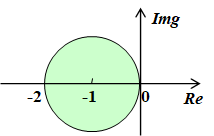
Thus it's only stable for some cases of stiff equation. When the negative $\lambda$ becomes smaller and get out of the region, it becomes not stable.

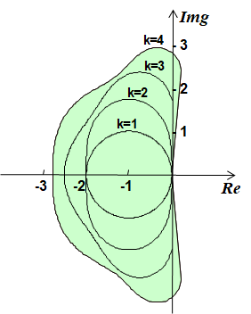
Similarly, for Runge-Kutta Order Four method (explicit), applying test equation, we have

\[ w_{i + 1} = \left(1 + H + \frac{H^2}{2} + \frac{H^3}{6} + \frac{H^4}{24}\right)w_i. \]

And the region is like

Let's consider some implicit method. Say Euler's implicit method, we have

\[ w_{i + 1} = \frac{1}{1 - H} w_i, \]

whose region is

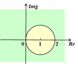
Thus it's A-stable.

Also, implicit Trapezoidal method and 2^nd-order Runge-Kutta implict method are A-stable, both with the difference equation

\[ w_{i + 1} = \frac{2 + H}{2 - H}w_i, \]

whose region is just right covers the left half-plane.

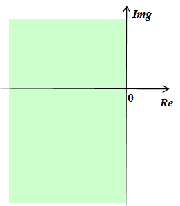
Thus an important intuitive is that implicit method is more stable than explicit method in the stiff discussion.

最后更新: 2023.11.21 17:00:13 CST
创建日期: 2022.11.10 01:04:43 CST