Sort

Suppose there is an array of comparable elements \(x_0, \dots x_{n - 1}\) and sort the array.

Property

When discussing various sort algorithms, we concerns the following properties.

Stability

Stability measures whether the algorithm change the relative order of the same elements.

Time Complexity

We consider the best time complexity, worst time complexity and average complexity.

Definition

An inversion in an array of numbers is any ordered pair \((i, j)\) with the property that

\[ i < j,\ \ A[i] > A[j]. \]

Theorem

The average number of inversions in an array of \(N\) distinct number is \(\dfrac{N(N - 1)}{4}\).

Theorem

• Any algorithm that sorts by exchanging adjacent elements requires \(\Omega(N^2)\) time on average.
• Any algorithm that sorts by comparison requires \(\Omega(N \log N)\) time on average.

Also, there are some sort algorithms not based on exchange.

Space Complexity

Space complexity considers the extra space the algorithm need.

Bubble Sort 冒泡排序

IterationIteration (Improved)Recursion

void BubbleSort(const int n, int a[]) {
    for (int i = n - 1; i >= 0; i --) {
        for (int j = 0; j < i; j ++) {
            if (a[j] > a[j + 1]) {
                Swap(a + j, a + j + 1);
            }
        }
    }
}

void BubbleSort(const int n, int a[]) {
    for (int i = n - 1, end = 0; i > 0; i = end, end = 0) {
        for (int j = 0; j < i; j ++) {
            if (a[j] > a[j + 1]) {
                Swap(a + j, a + j + 1);
                end = j;
            }
        }
    }
}

void BubbleSort(const int n, int a[]) {
    if (n == 0) {
        return;
    }
    for (int i = 0; i < n - 1; i ++) {
        if (a[i] > a[i + 1]) {
            Swap(a + i, a + i + 1);
        }
    }
    BubbleSort(n - 1, a);
}

Analysis

• Stable.
• Time complexity \(O(n^2)\).
• Space complexity \(O(1)\).

Insertion Sort 插入排序

IterationRecursion

void InsertionSort(const int n, int a[]) {
    int j;
    for (int i = 1; i < n; i ++) {
        int x = a[i];
        for (j = i - 1; j >= 0 && a[j] > x; j --) {
            a[j + 1] = a[j];
        }
        a[j + 1] = x;
    }
}

void InsertionSort(const int n, int a[]) {
    if (n == 0) {
        return;
    }
    InsertionSort(n - 1, a);
    int x = a[n - 1], j;
    for (j = n - 2; j >= 0 && a[j] > x; j --) {
        a[j + 1] = a[j];
    }
    a[j + 1] = x;
}

Analysis

• Stable.
• Time complexity
  • Avearge case \(O(n^2)\).
  • Best case \(O(n)\) (High Efficiency when it's almost in order).
  • When \(n \le 20\), insertion sort is the fastest.
• Space complexity \(O(1)\).

Selection Sort 选择排序

IterationRecursion

void InsertionSort(const int n, int a[]) {
    for (int i = 0; i < n - 1; i ++) {
       int idx = i;
       for (int j = i + 1; j < n; j ++) {
            idx = a[j] < a[idx] ? j : idx;
       }
       Swap(a + i, a + idx);
    }
}

int FindMin(int a[], const int begin, const int end) {
    int ret = begin;
    for (int i = begin + 1; i <= end; i++) {
        ret = a[i] < a[ret] ? i : ret;
    }
    return ret;
}

void Sort(int a[], const int begin, const int end) {
    if (begin == end) {
        return;
    }
    Swap(a + begin, a + FindMin(a, begin, end));
    Sort(a, begin + 1, end);
}

void SelectionSort(const int n, int a[]) {
    Sort(a, 0, n - 1);
}

Analysis

• Unstable.
• Time complexity \(O(n^2)\).
• Space complexity \(O(1)\).

Counting Sort 计数排序

#define m 10010 // (1)!
void CountingSort(const int n, int a[]) {
    int cnt[m], b[n];
    memset(cnt, 0, sizeof(cnt));
    for (int i = 0; i < n; i ++) {
        cnt[a[i]] ++;
    }
    for (int i = 0; i < m; i ++) {
        cnt[i] += cnt[i - 1];
    }
    for (int i = n - 1; i >= 0; i --) {
        b[cnt[a[i] --] = a[i];
    }
    memcpy(a, b, sizeof(a));
}

1. m is the upper bound of a[i].

Analysis

• Stable.
• Time complexity \(O(n + m)\), where \(m\) is the upper bound of \(a[i]\).
• Space complexity \(O(n + m)\).

Radix Sort 基数排序

typedef struct {
    int element;
    int key[K]; // (1)!
} ElementType;

void CountingSort(const int n, ElementType a[], int p, int cnt[], ElementType b[]) {
    memset(cnt, 0, sizeof(cnt));
    for (int i = 0; i < n; i ++) {
        cnt[a[i].key[p]] ++;
    }
    for (int i = 0; i < m[p]; i ++) {
        cnt[i] += cnt[i - 1];
    }
    for (int i = n - 1; i >= 0; i --) {
        b[cnt[a[i].key[p] --] = a[i];
    }
    memcpy(a, b, sizeof(a));
} 

void RadixSort(const int n, ElementType a[]) {
    int cnt[M]; // (2)!
    ElementType b[n];
    for (int i = k - 1; i >= 0; i --) {
        CountingSort(n, a, i, cnt, b);
    }
}

1. K is the number of keys.
2. M is the maximum of m[i], where m[i] is the upper bound of each key.

The most common keys for sorting integers are

• the digit number from high to low (left to right), which is called Most Significant Digit (MSD) sort.
• the digit number from low to high (right to left), which is called Least Significant Digit (LSD) sort.

In general, LSD is better than MSD.

Keys of LSDKeys of MSD

for (int i = 0; i < n; i ++) {
    for (int j = 0; j < K; j ++) {
        a[i].key[j] = (int)(a[i].element / pow(10, j)) % 10;
    }
}

for (int i = 0; i < n; i ++) {
    for (int j = 0; j < K; j ++) {
        a[i].key[j] = (int)(a[i].element / (pow(10, K - 1) / pow(10, j))) % 10;
    }
}

Analysis

• Stable unless the inner sort is unstable.
• Time complexity
  • If \(\max\{m_i\}\) is small, we can use Counting Sort as the inner sort, then the time complexity is \(O\left(nk + \sum\limits_{i = 1}^k m_i\right)\), where \(k\) is the number of keys, \(m_i\) is the upper bound of each key.
  • If \(\max\{m_i\}\) is large, we use the sort based on comparison of \(O(nk \log n)\) instead of Radix Sort.
• Space complexity \(O(n + \max\{m_i\})\).

Quick Sort 快速排序

void Sort(int a[], const int L, const int R) {
    if (L >= R) {
            return;
    }

    int rnd = L + rand() % (R - L); // (1)!
    int pos = L, cnt = 0;
    Swap(&a[L], &a[rnd]);
    for (int i = L + 1; i <= R; i ++) { // (2)!
        if (a[i] < a[L]) {
            pos ++;
            if (pos + cnt < i) {
                Swap(&a[pos], &a[cnt + pos]);
            }
            Swap(&a[i], &a[pos]);
            continue;
        }
        if (a[i] == a[L]) {
            cnt ++;
            Swap(&a[i], &a[cnt + pos]);
        }
    }
    Swap(&a[L], &a[pos]);

    Sort(a, L, pos - 1);
    Sort(a, pos + 1 + cnt, R);
}

void QuickSort(const int n, int a[]) {
    srand(time(NULL));
    Sort(a, 0, n - 1);
}

1. Different pivot picking strategies are discussed below.
2. This is a 3-way radix quicksort.

Analysis

• Unstable.
• Time complexity
  • Best and average cases \(O(n \log n)\).
  • Worst cases \(O(n^2)\).
    • Each pivot a[pos] is the maxima / minima.
    • Degenerate to list.
• Space complexity \(O(1)\).

Time Complexity

\[ T(N) = T(i) + T(N - i - 1) + cN. \]

• Worst Case

\[ T(N) = T(N - 1) + cN \Rightarrow T(N) = O(N^2), \]

• Best Case

\[ T(N) = 2T\left(\frac{N}{2}\right) + cN \Rightarrow T(N) = O(N\log N), \]

• Average Case

\[ T(N) = \frac2N\sum\limits_{j = 0}^{N - 1}T(j) + cN \Rightarrow T(N) = O(N\log N). \]

Pivot Picking Strategy

• A simple way is a[0].
• A random way, which is used above, is a[rnd], where rnd is a random number between L and R.

• Median-of-Three Paritioning a[mid], where mid = median(left, center, right).

  Code

  int MediamThree(int a[], const int L, const int R) {
      int mid = L + ((R - L) >> 1);
      if (a[L] > a[mid]) {
          Swap(a + L, a + mid);
      }
      if (a[L] > a[R]) {
          Swap(a + L, a + R);
      }
      if (a[mid] > a[R]) {
          Swap(a + mid, a + R);
      }
      assert(a[L] <= a[mid] && a[mid] <= a[R]);
      Swap(a[mid], a[R - 1]);
      return a[R - 1];
  }
  

Improvement

Suppose the value of pivot is v.

2-way Radix Quicksort

Scan from left and right respectively by two index (i, j), make the elements <= v on the left of i and the elements >= v on the right of j.

3-way Radix Quicksort

Partition the series into THREE parts: > m, < m and = m. It's efficient to deal with the cases of multiple identical values.

Merge Sort 归并排序

RecursionIteration

void Merge(int a[], const int L, const int mid, const int R, int temp[]) {
    int i = L, j = mid + 1;
    for (int k = L; k <= R; k ++) {
        if (i <= mid && (j > R || a[i] <= a[j])) {
            temp[k] = a[i];
            i ++;
        } else {
            temp[k] = a[j];
            j ++;
        }
    }
    memcpy(a + L, temp + L, (R - L + 1) * sizeof(int));
}

void Sort(int a[], const int L, const int R, int temp[]) {
    if (L == R) {
        return;
    }

    int mid = L + ((R - L) >> 1);
    Sort(a, L, mid, temp);
    Sort(a, mid + 1, R, temp);
    Merge(a, L, mid, R, temp);
}

void MergeSort(const int n, int a[]) {
    int temp[n];
    Sort(a, 0, n - 1, temp);
}

#define min(a, b) ((a) < (b) ? (a) : (b))

void Merge(int a[], const int L, const int mid, const int R, int temp[]) {
    int i = L, j = mid + 1;
        for (int k = L; k <= R; k ++) {
        if (i <= mid && (j > R || a[i] <= a[j])) {
            temp[k] = a[i];
            i ++;
        } else {
            temp[k] = a[j];
            j ++;
        }
    }
        memcpy(a + L, temp + L, (R - L + 1) * sizeof(int));
}

void MergeSort(const int n, int a[]) {
    int temp[n];
    for (int width = 1; width < n; width <<= 1) {
        for (int i = 0; i < n; i += width << 1) {
            Merge(a, i, min(n, i + width) - 1, min(n, i + (width << 1) - 1), temp);
        }
    }
}

Analysis

• Stable.
• Time complexity \(O(n \log n)\).
• Space complexity \(O(n)\).
• Better performance at parallel sort.

Time Complexity

\[ \begin{aligned} T(1) &= 1, \\ T(N) &= 2T\left(\frac{N}{2}\right) + O(N) \\ &= 2^k T\left(\frac{N}{2^k}\right) + k \cdot O(N) \\ &= N \cdot O(1) + \log N \cdot O(N) \\ &= O(N + N \log N). \end{aligned} \]

Bucket Sort 桶排序

#define m 10010 // (1)!

typedef struct _node {
    int element;
    struct _node *next;
} Node;
typedef struct {
    int size;
    Node *head;
} List;

void InsertionSort(List *list) { // (2)!
    for (Node *p = list->head->next, *q = list->head; p != NULL;) {
        bool flag = false;
        for (Node *r = list->head->next, *s = list->head; r != p; s = r, r = r->next) {
            if (r->element > p->element) {
                Node *temp = p;
                p = p->next;
                q->next = p;
                flag = true;

                s->next = temp;
                temp->next = r;
                break;
            }
        }
        if (flag == false) {
            q = p;
            p = p->next;
        }
    }
}

void BucketSort(const int n, int a[]) {
    int bucketNum = 6; // (3)!
    int bucketSize = (m + bucketNum - 1) / bucketNum;
    List **bucket = (List **)malloc(bucketNum * sizeof(List *));
    for (int i = 0; i < bucketNum; i ++) {
        bucket[i] = (List *)malloc(sizeof(List));
        bucket[i]->size = 0;
        bucket[i]->head = (Node *)malloc(sizeof(Node));
        bucket[i]->head->next = NULL;
    }

    for (int i = 0; i < n; i ++) {
        int pos = a[i] / bucketSize;
        bucket[pos]->size ++;
        Node *p = (Node *)malloc(sizeof(Node));
        p->element = a[i];
        p->next = bucket[pos]->head->next;
        bucket[pos]->head->next = p;
    }

    for (int i = 0, cnt = 0; i < bucketNum; i ++) {
        InsertionSort(bucket[i]);
        for (Node *p = bucket[i]->head->next; p != NULL; p = p->next) {
            a[cnt ++] = p->element;
        }
    }

    for (int i = 0; i < bucketNum; i ++) {
        for (Node *p = bucket[i]->head, *temp = NULL; p != NULL;) {
            temp = p;
            p = p->next;
            free(temp);
        }
        free(bucket[i]);
    }
    free(bucket);
}

1. m is the upper bound of a[i].
2. The inner sort is used insertion sort, and here is a list implementation of Insertion Sort.
3. bucketNum is the number of the bucket.

Analysis

• Similar to Radix Sort.
• Stable unless the inner sort is unstable.
• Time complexity
  • Average case \(O\left(n + k \cdot \left(\dfrac{n}{k}\right)^2 + k\right)\), where \(k\) is the number of the bucket.
  • Worst case \(O(n^2)\).
  • Large constant of time complexity.
• Space complexity \(O(n)\).

Heap Sort 堆排序

void MaxHeapify(int a[], int p, int size) { // (1)!
    while (p << 1 <= size) {
        int child = p << 1;
        if (child != size && a[child] < a[child + 1]) {
            child ++;
        }
        if (a[p] < a[child]) {
            Swap(a + p, a + child);
        } else {
            break;
        }
        p = child;
    }
}

void HeapSort(const int n, int a[]) {
    for (int i = n / 2 - 1; i >= 0; i --) { // (2)!
        MaxHeapify(a, i, n - 1);
    }
    for (int i = n - 1; i > 0; i --) {
            Swap(a, a + i);
        MaxHeapify(a, 0, i - 1);
    }
}

1. The same as PercolateDown() of implementation of heap.
2. The same as Build Heap.

Analysis

• Improvement of Selection Sort.
• Unstable.
• Time complexity \(O(n \log n)\).
• Space complexity \(O(1)\).
• Much cache miss and not based on partition, which means hard to parallel.

Theorem

The average number of comparisons used to heapsort a random permutation of N distinct items is \(2N \log N - O(N\log \log N)\).

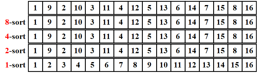
Shell Sort 希尔排序

Shell's IncrementShell's Increment (Simplified)Hibbard's Increment

void ShellSort(const int n, int a[]) {
    for (int step = n >> 1; step > 0; step >>= 1) {
        for (int start = 0; start < step; start ++) {
            for (int i = start; i < n; i += step) {
                int temp = a[i], j;
                for (j = i; j >= step; j -= step) {
                    if (temp < a[j - step]) {
                        a[j] = a[j - step];
                    } else {
                        break;
                    }
                }
                a[j] = temp;
            }
        }
    }
}

void ShellSort(const int n, int a[]) {
    for (int step = n >> 1; step > 0; step >>= 1) {
        for (int i = step; i < n; i += step) {
            int temp = a[i], j;
            for (j = i; j >= step; j -= step) {
                if (temp < a[j - step]) {
                    a[j] = a[j - step];
                } else {
                    break;
                }
            }
            a[j] = temp;
        }
    }
}

void ShellSort(const int n, int a[]) {
    int t = 1, step;
    while (t << 1 < n) {
        t <<= 1;
    }
    step = t - 1;

    while (step > 0) {
        for (int i = step; i < n; i += step) {
            int temp = a[i], j;
            for (j = i; j >= step; j -= step) {
                if (temp < a[j - step]) {
                    a[j] = a[j - step];
                } else {
                    break;
                }
            }
            a[j] = temp;
        }
        t >>= 1;
        step = t - 1;
    }
}

Analysis

• Improvement of Insertion Sort.
• Unstable.
• Time complexity
  • Depend on the increment sequence (example are discussed below).
  • Best case \(O(n)\).
  • Worst case \(\Theta(n^2)\).
  • Best worst case that are known is \(O(n \log^2 n)\).
• Space complexity \(O(1)\).
• Much cache miss and not based on partition, which means hard to parallel.

Choice of Increment Sequence

Shell's Increment Sequence

\[ h_t = \left\lfloor \frac{N}{2} \right\rfloor,\ \ h_k = \left\lfloor \frac{h_{k + 1}}{2} \right\rfloor. \]

Theorem

The worst case running time of Shell Sort using Shell's increment sequence is \(\Theta(N^2)\).

Worst Case of Shell's Increment Sequence

Hibbard's Increment Sequence

\[ h_k = 2^k - 1. \]

Theorem

The worst case running time of Shell Sort using Hibbard's increment sequence is \(\Theta\left(N^{\frac{3}{2}}\right)\).

Conjectures

\[ T_{avg-Hibbard}(N) = O\left(N^{\frac54}\right). \]

Conjectures: Sedgewick's Best Sequence

Sedgewick’s best sequence is \(\{1, 5, 19, 41, 109, \dots\}\) in which the terms are either of the form \(9 \times 4^i - 9 \times 2^i + 1\) or \(4^i – 3 \times 2^i + 1\).

\[ T_{avg}(N) = O\left(N^{\frac76}\right),\ \ T_{worst}(N) = O\left(N^{\frac43}\right). \]

---

最后更新: 2023.11.21 17:00:13 CST
创建日期: 2022.11.10 01:04:43 CST