Chapter 8 | Approximation Theory

Abstract

Target

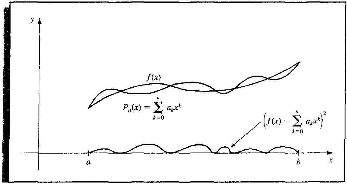
Given \(x_1, \dots, x_m\) and \(y_1, \dots, y_m\) sampled from a funciton \(y = f(x)\), or the continuous function \(f(x)\), \(x \in [a, b]\) itself, find a simpler function \(P(x) \approx f(x)\).

Measurement of Error

• (Minimax) minimize
  • (discrete) \(E_\infty = \max\limits_{1 \le i \le m}|P(x_i) - y_i|\).
  • (continuous) \(E_\infty = \max\limits_{a \le x \le b}|P(x) - f(x)|\).
• (Absolute Deviation) minimize
  • (discrete) \(E_1 = \sum\limits_{i = 1}^{m}|P(x_i) - y_i|\).
  • (continuous) \(E_1 = \int\nolimits_{a}^{b}|P(x) - f(x)|dx\).
• (Least Squares Method) minimize
  • (discrete) \(E_2 = \sum\limits_{i = 1}^{m}|P(x_i) - y_i|^2\).
  • (continuous) \(E_2 = \int\nolimits_{a}^{b}|P(x) - f(x)|^2dx\).

In this course, we only discuss the minimax and least square parts, and only make \(P(x)\) a polynomial function.

General Least Squares Approximation

Definition 8.0

\(w\) is called a weight function if

• (discrete)

  \[ \forall\ i \in \mathbb{N},\ \ w_i > 0. \]

• (continuous) \(w\) is an integrable function and on the interval \(I\),

  \[ \forall\ x \in I,\ \ w(x) \ge 0, \]
  \[ \forall\ I' \subseteq I,\ \ w(x) \not\equiv 0. \]

Considering the weight function, the least square method can be more general as below.

• (discrete) \(E_2 = \sum\limits_{i = 1}^{m}w_i|P(x_i) - y_i|^2\).
• (continuous) \(E_2 = \int\nolimits_{a}^{b}w(x)|P(x) - f(x)|^2dx\).

Discrete Least Squares Approximation

Target

Approximate a set of data \(\{(x_i, y_i) | i = 1, 2, \dots, m\}\), with an algebraic polynomial

\[ P_n(x) = a_nx^n + a_{n - 1}x^{n - 1} + \cdots + a_1x + a_0, \]

of degree \(n < m - 1\) (in most case \(n \ll m\)), with the least squares measurement, w.r.t. and weight function \(w_i \equiv 1\).

Solution

\[ \begin{aligned} E_2 &= \sum\limits_{i = 1}^m (y_i - P_n(x_i))^2 \\ &= \sum\limits_{i = 1}^m y_i^2 - 2\sum\limits_{i = 1}^m P_n(x_i)y_i + \sum\limits_{i = 1}^m P_n^2(x_i) \\ &= \sum\limits_{i = 1}^m y_i^2 - 2\sum\limits_{i = 1}^m \left(\sum\limits_{j = 0}^n a_jx_i^j\right)y_i + \sum\limits_{i = 1}^m \left(\sum\limits_{j = 0}^n a_jx_i^j \right)^2 \\ &= \sum\limits_{i = 1}^m y_i^2 - 2\sum\limits_{j = 0}^n a_j \left( \sum\limits_{i = 1}^m y_i x_i^j \right) + \sum\limits_{j = 0}^n \sum\limits_{k = 0}^n a_ja_k \left(\sum\limits_{i = 1}^m x_i^{j + k} \right). \end{aligned} \]

The necessary condition to minimize \(E_2\) is

\[ 0 = \frac{\partial E_2}{\partial a_j} = -2 \sum\limits_{i = 1}^m y_i x_i^j + 2 \sum\limits_{k = 0}^n a_k \sum\limits_{i = 1}^m x_i^{j + k}. \]

Then we get the \(n + 1\) normal equations with \(n + 1\) unknown \(a_j\),

\[ \sum\limits_{k = 0}^n a_k \sum\limits_{i = 1}^m x_i^{j + k} = \sum\limits_{i = 1}^m y_i x_i^j. \]

Let \(b_k = \sum\limits_{i = 1}^m x_i^k\) and \(c_k = \sum\limits_{i = 1}^m y_i x_i^k\), we can represent the normal equations by

\[ \begin{bmatrix} b_{0 + 0} & \cdots & b_{0 + n} \\ \vdots & \ddots & \vdots \\ b_{n + 0} & \cdots & b_{n + n} \end{bmatrix} \begin{bmatrix} a_0 \\ \vdots \\ a_n \end{bmatrix} = \begin{bmatrix} c_0 \\ \vdots \\ c_n \end{bmatrix} \]

Theorem 8.0

Normal equations have a unique solution if \(x_i\) are distinct.

Proof

Suppose \(X\) is an \(n + 1 \times m\) Vandermonde Matrix, which is

\[ X = \begin{bmatrix} 1 & x_1 & x_1^2 & \cdots & x_1^n \\ 1 & x_2 & x_2^2 & \cdots & x_2^n \\ \vdots & \vdots & \ddots & \vdots \\ 1 & x_m & x_m^2 & \cdots & x_m^n \\ \end{bmatrix}, \]

and let \(\mathbf{y} = (y_1, y_1, \cdots, y_m)^T\).

Then the normal equations can be represented by (notice the dimension of matrices and vectors),

\[ X X^T \mathbf{a} = X \mathbf{y}. \]

Since \(x_i\) are distinct, \(X\) is a column full rank matrix, namely

\[ \text{rank}(X) = n + 1. \]

Since \(x_i \in \mathbb{R}\), thus

\[ \text{rank}(X X^T) = \text{rank}(X) = n + 1. \]

Hence the normal equations have a unique solution.

Logarithmic Linear Least Squares

To approximate by the function of the form

\[ y = be^{ax}, \]

or

\[ y = bx^a, \]

we can consider the logarithm of the equation by

\[ \ln y = \ln b + ax, \]

and

\[ \ln y = \ln b + a \ln x. \]

Note

It's a simple algrebric transformation. But we should point out that it minimize the logarithmic linear least squares, but not linear least squares.

Just consider the arguments to minimize the following two errors,

\[ E = \sum\limits_{i = 1}^m (y_i - be^{ax_i})^2, \]

and

\[ E' = \sum\limits_{i = 1}^m (\ln y - (\ln b + ax))^2, \]

they are slightly different actually.

Continuous Least Squares Approximation

Now we consider the continuous function instead of discrete points.

Target

Approxiate function \(f \in C[a, b]\), with an algebraic polynomial

\[ P_n(x) = a_nx^n + a_{n - 1}x^{n - 1} + \cdots + a_1x + a_0, \]

with the least squares measurement, w.r.t the weight function \(w(x) \equiv 1\).

Solution

Problem

Similarly to the discrete situation, we can derive the normal equations by making

\[ 0 = \frac{\partial E}{\partial a_j}, \]

and we get the normal equations

\[ \sum\limits_{k = 0}^n a_k \int_{a}^{b} x^{j + k} dx = \int_{a}^{b} x^j f(x)dx. \]

However, notice that

\[ \int_{a}^{b} x^{j + k} dx = \frac{b^{j + k + 1} - a^{j + k + 1}}{j + k + 1}. \]

Thus the coefficient of the linear system is a Hilbert matrix, which has a large conditional number. In actual numerical calculation, this gives a large roundoff error.

Another disadvantage is that we can not easily get \(P_{n + 1}(x)\) from \(P_{n}(x)\), similarly with the discussion of Lagrange interpolation.

Hence we introduce a different solution based on the concept of orthogonal polynomials.

Definition 8.1

The set of function \(\{\varphi_0(x), \dots, \varphi_n(x)\}\) is linearly independent on \([a, b]\) if, whenever

\[ \forall\ x \in [a, b], c_0\varphi_0(x) + c_1\varphi_1(x) + \cdots + c_n\varphi_n(x) = 0 \]

we have \(c_0 = c_1 = \cdots = c_n = 0\). Otherwise it's linearly dependent.

Theorem 8.1

If \(\text{deg}(\varphi_j(x)) = j\), then \(\{\varphi_0(x), \dots, \varphi_n(x)\}\) is linearly independent on any interval \([a, b]\).

Theorem 8.2

\(\Pi_n\) is the linear space spanned by \(\{\varphi_0(x), \dots, \varphi_n(x)\}\), where \(\{\varphi_0(x), \dots, \varphi_n(x)\}\) is linear independent, and \(\Pi_n\) is the set of all polynomials of degree at most n.

Definition 8.2

For the linear independent set \(\{\varphi_0(x), \dots, \varphi_n(x)\}\), \(\forall P(x) \in \Pi_n\), \(P(x) = \sum\limits_{j = 0}^n \alpha_j \varphi_j(x)\) is called a generalized polynomial.

Definition 8.3

Inner product w.r.t the weight function \(w\) is defined and denoted by

• (discrete) \((f, g) = \sum\limits_{i = 1}^{m} w_i f(x_i)g(x_i)\)
• (continuous) \((f, g) = \int\nolimits_{a}^{b} w(x) f(x) g(x) dx\).

\(\{\varphi_0(x), \dots, \varphi_n(x)\}\) is an orthogonal set of functions for the interval \([a,b]\) w.r.t the weight function \(w\) if

\[ (\varphi_j, \varphi_k) = \left\{ \begin{aligned} & 0, && j \ne k, \\ & \alpha_k > 0, && j = k. \end{aligned} \right. \]

In addition, if \(\alpha_k = 1\), then the set is orthonormal （单位正交）.

Motivation of Orthogonality

Considering \(w(x)\), then the normal equations can be represented by

\[ \int_a^b w(x)f(x)\varphi_j(x)dx = \sum\limits_{k = 0}^n a_k \int_a^b w(x)\varphi_k(x)\varphi_j(x)dx. \]

If we define the orthogonal set of functions as above, the equations reduce to

\[ \int_a^b w(x)f(x)\varphi_j(x)dx = a_j \alpha_j. \]

Theorem 8.3

\(\{\varphi_0(x), \dots, \varphi_n(x)\}\) is an orthogonal set of functions on the interval \([a, b]\) w.r.t. the weight function \(w\), then the least squares approximation to \(f\) on \([a, b]\) w.r.t. \(w\) is

\[ P(x) = \sum\limits_{k = 0}^n a_k \varphi_k(x), \]

where, for each \(k = 0, 1, \dots, n\),

\[ a_k = \frac{\int_a^b w(x) \varphi_k(x)f(x)dx}{\int_a^b w(x) \varphi_k^2(x)dx} = \frac{(\varphi_k, f)}{(\varphi_{k}, \varphi_{k})} = \frac{(\varphi_k, f)}{\alpha_k}. \]

Base on the Gram-Schmidt Process, we have the following theorem to construct the orthogonal polynomials on \([a, b]\) w.r.t a weight function \(w\).

Theorem 8.4

The set of polynomial functions \(\{\varphi_0(x), \dots, \varphi_n(x)\}\) defined in the following way is orthogonal on \([a, b]\) w.r.t. the weight function \(w\).

\[ \begin{aligned} & \varphi_0(x) \equiv 1,\ \varphi_1(x) = x - B_1, \\ & \varphi_k(x) = (x - B_k) \varphi_{k - 1}(x) - C_k \varphi_{k - 2}(x), k \ge 2. \\ \end{aligned} \]

where

\[ B_k = \frac{(x\varphi_{k - 1}, \varphi_{k - 1})}{\varphi_{k - 1}, \varphi_{k - 1}},\ \ C_k = \frac{(x\varphi_{k - 1}, \varphi_{k - 2})}{\varphi_{k - 2}, \varphi_{k - 2}}. \]

Minimax Approximation

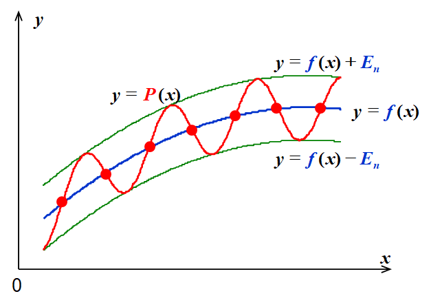
The minimax approximation to minimize \(||P - f||_\infty||\) has the following properties.

Proposition

• If \(f \in C[a, b]\) and \(f\) is not a polynomial of degree \(n\), then there exists a unique polynomial \(P(x)\) s.t. \(||P - f||\infty\) is minimized.
• \(P(x)\) exists and must have both \(+\) and \(-\) deviation points.

• (Chebyshev Theorem) The \(n\) degree \(P(x)\) minimizes \(||P - f||_\infty\) \(\Leftrightarrow\) \(P(x)\) has at least \(n + 2\) alternating \(+\) and \(-\) deviation points w.r.t. \(f\). That is, there is a set of points \(a \le t_1 < \dots < t_{n + 2} \le b\) (called the Chebyshev alternating sequence) s.t.

  \[ P(t_k) - f(t_k) = (-1)^k||P - f||_\infty. \]

Here we introduce Chebyshev polynomials to deal with \(E_\infty\) error, and by the way, we can use it to economize the power series.

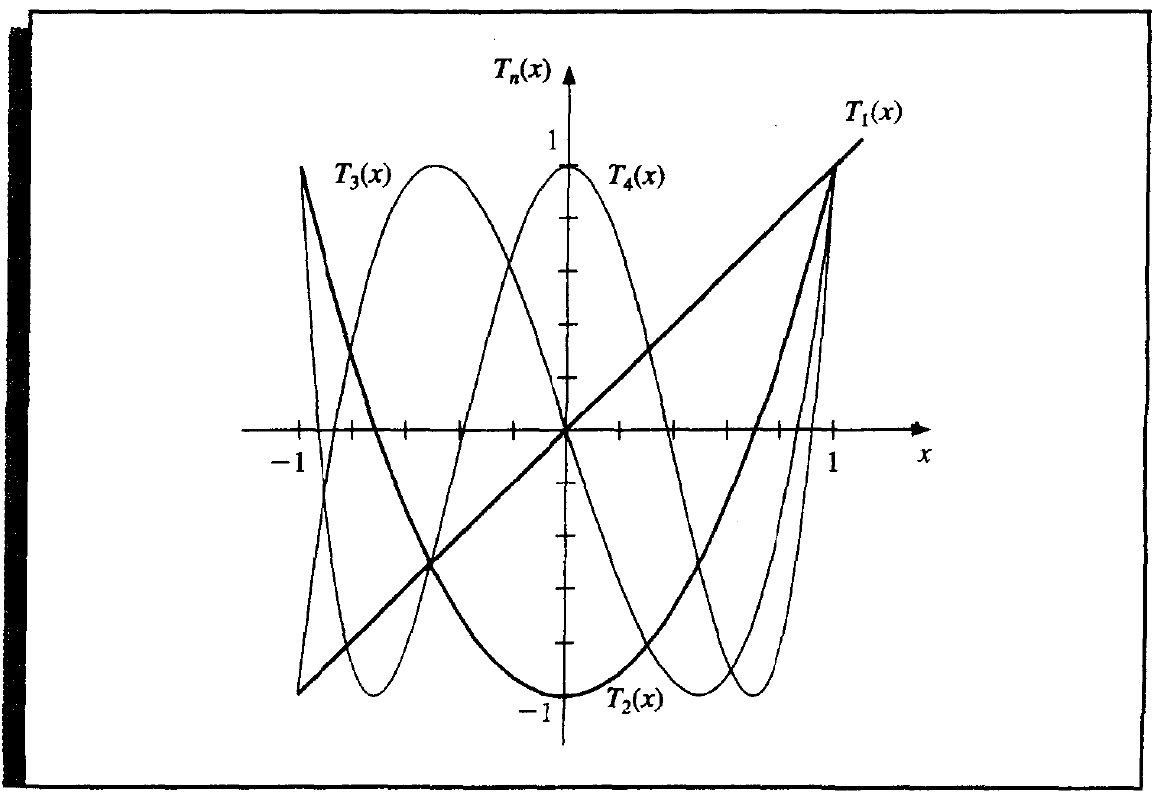
Chebyshev Polynomials

Chebyshev polynomials are defined concisely by

\[ T_n(x) = \cos(n \arccos x), \]

or equally defined recursively by

\[ \begin{aligned} & T_0(x) = 1,\ T_1(x) = x, \\ & T_{n + 1}(x) = 2x T_{n}(x) - T_{n - 1}(x). \end{aligned} \]

Property

• \(\{T_n(x)\}\) are orthogonal on \((-1, 1)\) w.r.t the weight function

  \[ w(x) = \frac{1}{\sqrt{1 - x^2}}. \]
  \[ (T_n, T_m) = \int_{-1}^1 \frac{T_n(x)T_m(x)}{\sqrt{1 - x^2}}dx = \left\{ \begin{aligned} & 0, && n \ne m, \\ & \pi, && n = m = 0, \\ & \frac{\pi}{2}, && n = m \ne 0. \end{aligned} \right. \]

• \(T_n(x)\) is a polynomial of degree \(n\) with the leading coefficient \(2^{n - 1}\).

• \(T_n(x)\) has \(n\) zero points at

  \[ \bar{x}_k = \cos \left(\frac{2k-1}{2n}\pi\right),\ k = 1, 2, \dots, n. \]

• \(T_n(x)\) has extrema at

  \[ \bar{x}'_k = \cos \frac{k\pi}n \text{, with } T(\bar{x}'_k) = (-1)^k,\ k = 1, 2, \dots, n. \]

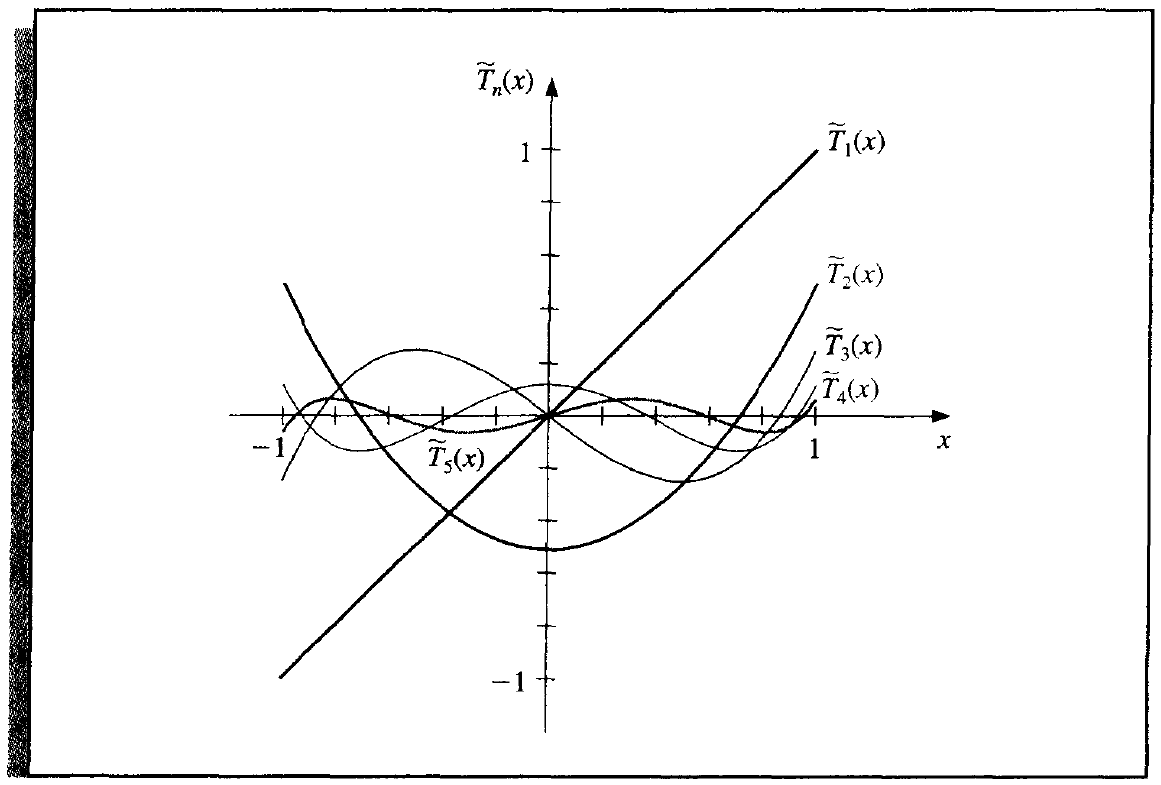
Monic Chebyshev Polynomials

Monic chebyshev polynomials are defined by

\[ \tilde T_0(x) = 1,\ \tilde T_n(x) = \frac{1}{2^{n - 1}} T_n(x). \]

The following is an important theorem for the position of Chebyshev polynomials.

Theorem 8.5

\[ \frac{1}{2^{n - 1}} = \max\limits_{x \in [-1, 1]}|\tilde T_n(x)| \le \max\limits_{x \in [-1, 1]}|P_n(x)|,\ \forall\ P_n(x) \in \tilde \Pi_n, \]

where \(\tilde \Pi_n\) denotes the set of all monic polynomials of degree n.

From theorem 8.5, we can answer where to place interpolating points to minimize the error in Lagrange interpolation. Recap that

\[ R(x) = f(x) - P(x) = \frac{f^{n + 1}(\xi)}{(n + 1)!}\prod\limits_{i = 0}^{n}(x - x_i). \]

To minimize \(R(x)\), since there is no control over \(\xi\), so we only need to minimize

\[ |w_n(x)| = \left|\prod\limits_{i = 0}^{n}(x - x_i)\right|. \]

Since \(w_n(x)\) is a monic polynomial of degree \((n + 1)\), we can obtain minimum when \(w_n(x) = \tilde T_{n + 1}(x)\).

To make it equal, we can simply make their zero points equal, namely

\[ x_k = \bar{x}_{k + 1} = \cos \frac{2k + 1}{2(n + 1)}\pi. \]

Corollary 8.6

\[ \max\limits_{x \in [-1, 1]} |f(x) - P(x)| \le \frac{\max\limits_{x \in [-1, 1]}\left|f^{(n + 1)}(x)\right|}{2^n (n + 1)!}. \]

Solution of Minimax Approximation

Now we come back to the minimax approximation. To minimize

\[ E_\infty = \max\limits_{a \le x \le b}|P(x) - f(x)|, \]

with a polynomial of degree \(n\) on the interval \([a, b]\), we need the following steps.

Step.1 Find the roots of \(T_{n + 1}(t)\) on the interval \([-1, 1]\), denoted by \(t_0, \dots, t_n\).

Step.2 Extend it to the interval \([a, b]\) by

\[ x_i = \frac12[(b - a)t_i + a + b]. \]

Step.3 Substitue \(x_i\) into \(f(x)\) to get \(y_i\).

Step.4 Compute the Langrange polynomial \(P(x)\) of the interpolating points \((x_i, y_i)\).

---

Ecomomization of Power Series

Chebyshev polynomials can also be used to reduce the degree of an approximating polynomials with a minimal loss of accuracy.

Consider approximating

\[ P_n(x) = a_nx^n + a_{n - 1}x^{n - 1} + \cdots + a_1x + a_0 \]

on [-1, 1].

Then the target is to minimize

\[ \max_{x\in[-1,1]}|P_n(x) - P_{n - 1}(x)|. \]

Solution

Since \(\frac{1}{a_n}(P_n(x) - P_{n - 1}(x))\) is monic, thus

\[ \max_{x\in[-1,1]}\left|\frac{1}{a_n}((P_n(x) - P_{n - 1}(x))\right| \ge \frac{1}{2^{n - 1}}. \]

Equality occurs when

\[ \frac{1}{a_n}((P_n(x) - P_{n - 1}(x)) = \tilde T_n(x). \]

Thus we can choose

\[ P_{n - 1}(x) = P_n(x) - a_n \tilde T_n(x) \]

with the minimum error value of

\[ \max_{x\in[-1,1]}|P_n(x) - P_{n - 1}(x)| = |a_n| \max_{x\in[-1,1]}\left|\frac{1}{a_n}((P_n(x) - P_{n - 1}(x))\right| = \frac{|a_n|}{2^{n - 1}}. \]

---

最后更新: 2023.11.21 17:00:13 CST
创建日期: 2022.11.10 01:04:43 CST