Lecture 3 Image Processing

Image Processing

Common Processs of Images:

Incresing contrast, Invert, Blur, Sharpen, Edge Detection ...

Convolution

• Continous 1-D form,

\[ (f * g)(x) = \int_{-\infty}^\infty f(y)g(x-y)dy. \]

• Discrete 2D form,

\[ (f * g)(x) = \sum_{i, j =-\infty}^\infty f(i, j)g(x - i, y - j). \]

Gaussian Blur

We define thb 2D Gaussian function as below,

\[ \large f(i, j) = \frac{1}{2\pi\sigma^2}e^{-\frac{i^2 + j^2}{2\sigma^2}}. \]

Process of Gaussian Blur

1. Define a window size (commmly a square, say \(n \times n\), and let \(r = \lfloor n / 2 \rfloor\)).
2. Select a point, say \((x, y)\) and then put a window around it.

3. Apply the Gaussian function at each point in the window, and sum them up, namely

   \[ G(x, y) = \sum\limits_{i = x - r}^{x + r}\sum\limits_{j = y - r}^{y + r}f(i,j). \]

4. Then the 「blurred」 value of point \((x, y)\) is \(G(x, y)\).

Sharpen

An example of kernel matrix

\[ f = \begin{bmatrix} 0 & -1 & 0 \\ -1 & 5 & -1 \\ 0 & -1 & 0 \end{bmatrix} \]

An insight

Let \(I\) be the original image, then the sharpen image can be consider as

\[ I' = I + (I - \text{blur}(I)), \]

where \(I - \text{blur}(I)\) can be regarded as the high frequency part of content.

Extract Gradients

Two examples of kernel matrices

• \(f = \begin{bmatrix} -1 & 0 & 1 \\ -2 & 0 & 2 \\ -1 & 0 & 1\end{bmatrix}\) extracts horizontal gradients.
• \(f = \begin{bmatrix} -1 & -2 & -1 \\ 0 & 0 & 0 \\ 1 & 2 & 1 \end{bmatrix}\) extracts vertical gradients.

Bilateral Filters

Feature

• Kernel depends on image content.
• Better performance but lower efficiency.

A trick: Separable Filter

Definition

A filter is separable if it can be wriiten as the outer product of two other filters.

Example

\[ \frac19 \begin{bmatrix} 1 & 1 & 1\\ 1 & 1 & 1\\ 1 & 1 & 1 \end{bmatrix} = \frac13 \begin{bmatrix} 1 \\ 1 \\ 1 \end{bmatrix} \times \frac13 \begin{bmatrix} 1 & 1 & 1 \end{bmatrix} \]

Purpose / Advantages: speed up the calculation.

Image Sampling

Basic Idea

Down-sampling → Reducing image size.

Aliasing

• Aliasing is the artifacts due to sampling.
• Higher frequencies need faster sampling.
• Undersampling creates frequency aliases.

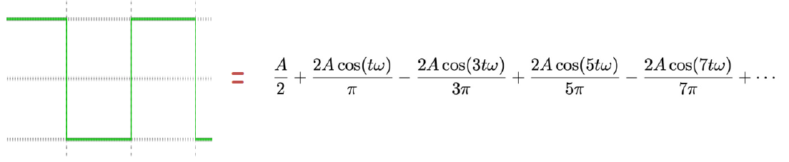
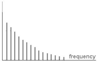
Fourier Transform

Simly put, fourier transform represents a function as a weighted sum of sines and cosines, where the sines and consines are in various frequencies.

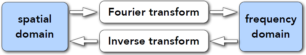
Convolution Theorem

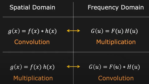
Now we can consider sampling and aliasing from the view of Fourier Transform (FT) ...

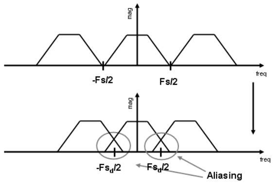
Sampling and Aliasing From FT

Sampling is repeating frequency contents. Aliasing is mixed frequency contents.

Method to reduce aliasing

• Increase sampling rate

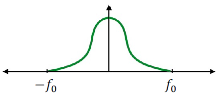
  Nyquist-Shannon theorem

  the signal can be perfectly reconstructed if sampled with a frequency larger than \(2f_0\).

  

• Anti-aliasing

  • Filtering → Sampling.

    

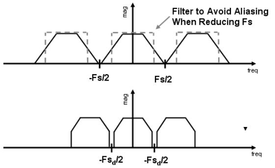
Example

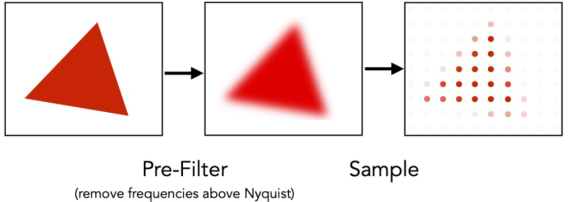
Image Magnification

Basic Idea

Up-sampling is Inverse of down-sampling.

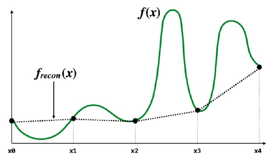
An important method: Interpolation.

1D Interpolation

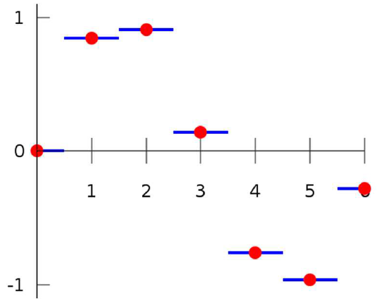
• Nearest-neighbour Interpolation

  • Feature: Not continuous; Not smooth.

    

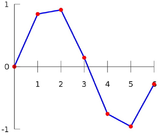
• Linear Interpolation

  • Feature: Continuous; Not smooth.

    

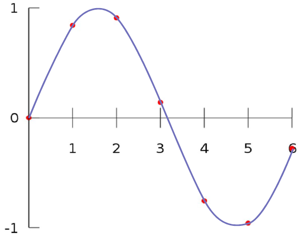
• Cubic Interpolation

  • Feature: Continuous; Smooth.

    

2D Interpolation

(similar to 1D cases)

• Nearest-neighbour Interpolation
• Bilinear Interpolation
  • define \(\text{lerp}(x, v_0,v_1) = v_0 + x(v_1 - v_0)\).
  • Suppose the point in the rectangle surrounded by four points are \(u_{00},u_{01},u_{10},u_{11}\).
  • then \(f(x, y) = \text{lerp}(t, u_0, u_1)\), where \(u_0 = \text{lerp}(s, u_{00}, u_{10})\) and \(u_1 = \text{lerp}(s, u_{01}, u_{11})\).
• Bicubic Interpolation
  

Super-Resolution

Remains

Change Aspect Ratio

Remains

---

最后更新: 2023.11.21 17:00:13 CST
创建日期: 2022.11.09 00:35:37 CST