Chapter 3 | Interpolation and Polynomial Approximation
Lagrange Interpolation
Suppose we have function \(y = f(x)\) with the given points \((x_0, y_0), (x_1, y_1), \dots, (x_n, y_n)\), and then construct a relatively simple approximating function \(g(x) \approx f(x)\).
Theorem 3.0
If \(x_0, x_1, \dots, x_n\) are \(n + 1\) distinct numbers and \(f\) is a function with given values \(f(x_0), \dots, f(x_n)\), then a unique polynomial \(P(x)\) of degree at most \(n\) exists with
and
where, for each \(k = 0, 1, \dots, n\),
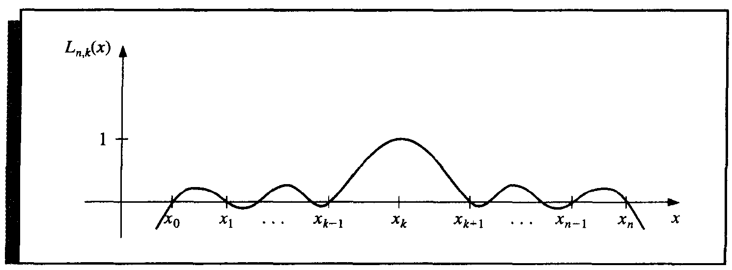
\(L_{n, k}(x)\) is called the n th Lagrange interpolating polynomial.
Proof
First we prove for the structure of function \(L_{n, k}(x)\).
From the definition of \(P(x)\), \(L_{n, k}(x)\) has the following properties.
- \(L_{n, k}(x_i) = 0\) when \(i \ne k\).
- \(L_{n, k}(x_k) = 1\).
To satisfy the first property, the numerator of \(L_{n, k}(x)\) contains the term
To satisfy the second property, the denominator of \(L_{n, k}(x)\) must be equal to the numerator at \(x = x_k\), thus
For uniqueness, we prove by contradition. If not, suppose \(P(x)\) and \(Q(x)\) both satisfying the conditions, then \(D(x) = P(x) - Q(x)\) is a polynomial of degree \(\text{deg}(D(x)) \le n\), but \(D(x)\) has \(n + 1\) distinct roots \(x_0, x_1, \dots, x_n\), which leads to a contradiction.
Theorem 3.1
If \(x_0, x_1, \dots, x_n\) are \(n + 1\) distinct numbers in the interval \([a, b]\) and \(f \in C^{n + 1}[a, b]\). \(\forall x \in [a, b], \exists \xi \in [a, b], s.t.\)
where \(P(x)\) is the Lagrange interpolating polynomial. And
is the truncation error.
Proof
Since \(R(x) = f(x) - P(x)\) has at least \(n + 1\) roots, thus
For a fixed \(x \ne x_k\), define \(g(t)\) in \([a, b]\) by
Since \(g(t)\) has \(n + 2\) distinct roots \(x, x_0, \dots, x_n\), by Generalized Rolle's Theorem, we have
Namely,
Thus
Example
Suppose a table is to be prepared for the function \(f(x) = e^x\) for \(x\) in \([0, 1]\). Assume that each entry of the table is accurate up to 8 decimal places and the step size is \(h\). What should \(h\) be for linear interpolation to give an absolute error of at most \(10^{-6}\)?
Solution.
Thus let \(\dfrac{eh^2}{8} \le 10^{-6}\), we have \(h \le 1.72 \times 10^{-3}\). To make \(N = \dfrac{(1 - 0)}{h}\) an integer, we can simply choose \(h = 0.001\).
Extrapolation
Suppose \(a = \min\limits_i \{x_i\}\), \(b = \max\limits_i \{x_i\}\). Interpolation estimates value \(P(x)\), \(x \in [a, b]\), while Extrapolation estimates value \(P(x)\), \(x \notin [a, b]\).
- In genernal, interpolation is better than extrapolation.
Neville's Method
Motivation: When we have more interpolating points, the original Lagrange interpolating method should re-calculate all \(L_{n, k}\), which is not efficient.
Definition 3.0
Let \(f\) be a function defined at \(x_0, x_1, \dots, x_n\), and suppose that \(m_1, \dots, m_k\) are \(k\) distinct integers with \(0 \le m_i \le n\) for each \(i\). The Lagrange polynomial that agrees with \(f(x)\) at the \(k\) points denoted by \(P_{m_1, m_2, \dots, m_k}(x)\).
Thus \(P(x) = P_{0, 1, \dots, n}(x)\), where \(P(x)\) is the n th Lagrange polynomials that interpolate \(f\) at \(k + 1\) points \(x_0, \dots, x_k\).
Theorem 3.2
Let \(f\) be a function defined at \(x_0, x_1, \dots, x_n\), and \(x_i \ne x_j\), then
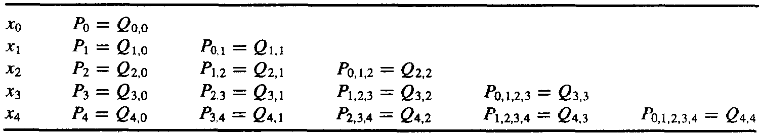
Denote that
then from Theorem 3.2, the interpolating polynomials can be generated recursively.
Newton Interpolation
Differing from Langrange polynomials, we try to represent \(P(x)\) by the following form:
Definition 3.1
\(f[x_i] = f(x_i)\) is the zeroth divided difference w.r.t. \(x_i\).
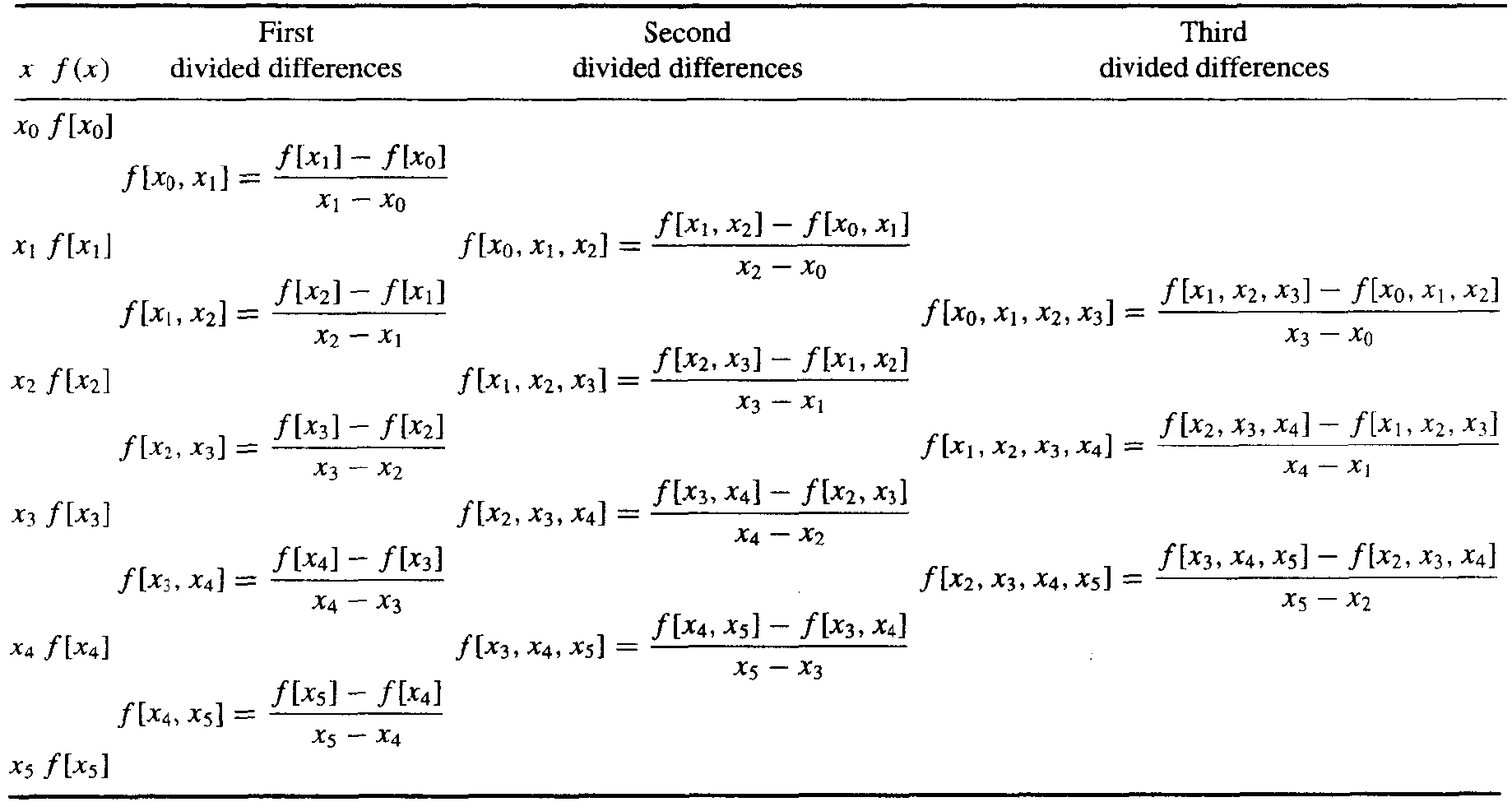
The k th divided difference w.r.t. \(x_i, x_{i + 1}, x_{i + k}\) is defined recursively by
Then we derive the Newton's interpolatory divided-difference formula
And the divided difference can be generated as below, which is similar to Neville's Method.
Theorem 3.3
If \(x_0, x_1, \dots, x_n\) are \(n + 1\) distinct numbers in the interval \([a, b]\) and \(f \in C^{n + 1}[a, b]\). \(\forall x \in [a, b], \exists \xi \in [a, b], s.t.\)
where \(N(x)\) is the Newton's interpolatory divided-difference formula. And
is the truncation error.
Proof
By definition of divided difference, we have
then compute
i.e.
Note
Since the uniqueness of n-th interpolating polynomial,
- \(N(x) \equiv P(x)\).
-
They have the same truncation error, which is
\[ f[x, x_0, \dots, x_n]\prod\limits_{i = 0}^n (x - x_i) = \frac{f^{(n + 1)}(\xi)}{(n + 1)!}\prod\limits_{i = 0}^n (x - x_i). \]
Theorem 3.4
Suppose that \(f \in C^n[a, b]\) and \(x_0, x_1, \dots, x_n\) are distinct numbers in \([a, b]\). Then \(\exists\ \xi \in (a, b)\), s.t.
Special Case: Equal Spacing
Definition 3.2
Forward Difference
Backward Difference
Property of Forward / Backward Difference
- Linearity \(\Delta (af(x) + bg(x)) = a \Delta f + b \Delta g\).
-
If \(\text{deg}(f(x)) = m\), then
\[ \text{deg}\left(\Delta^kf(x)\right) = \left\{ \begin{aligned} & m - k, & 0 \le k \le m, \\ & 0, & k > m. \end{aligned} \right. \] -
Decompose the recursive definition,
\[ \begin{aligned} \Delta^n f_k &= \sum\limits_{j = 0}^n (-1)^j \binom{n}{j} f_{n + k - j}, \\ \nabla^n f_k &= \sum\limits_{j = 0}^n (-1)^{n - j} \binom{n}{j} f_{j + k - n}. \end{aligned} \] -
Vice versa,
\[ f_{n + k} = \sum\limits_{j = 0}^n \binom{n}{j} \Delta^j f_k. \]
Suppose \(x_0, x_1, \dots x_n\) are equally spaced, namely \(x_i = x_0 + ih\). And let \(x = x_0 + sh\), then \(x - x_i = (s - i)h\). Thus
is called Newton forward divided-difference formula.
From mathematical induction, we can derive that
Thus we get the Newton Forward-Difference Formula
Inversely, \(x = x_n + sh\), then \(x - x_i = (s + n - i)h\), Thus
is called Newton backward divided-difference formula.
From mathematical induction, we can derive that
Thus we get the Newton Backward-Difference Formula
Hermit Interpolation
Definition 3.3
Let \(x_0, x_1, \dots, x_n\) be \(n + 1\) distinct numbers in \([a, b]\) and \(m_i \in \mathbb{N}\). Suppose that \(f \in C^m[a, b]\), where \(m = \max \{m_i\}\). The osculating polynomial approximating \(f\) is the polynomial \(P(x)\) of least degree such that
From definition above, we know that when \(m_i = 0\) for each \(i\), it's the n-th Lagrange polynomial. And the cases that \(m_i = 1\) for each \(i\), then it's Hermit Polynomials.
Theorem 3.5
If \(f \in C^1[a, b]\) and \(x_0, \dots, x_n \in [a, b]\) are distinct, the unique polynomial of least degree agreeing with \(f\) and \(f'\) at \(x_0, \dots, x_n\) is the Hermit Polynomial of degree at most \(\bf 2n + 1\) defined by
where
and
Moreover, if \(f \in C^{2n + 2}[a, b]\), then \(\exists\ \xi \in (a, b)\), s.t.
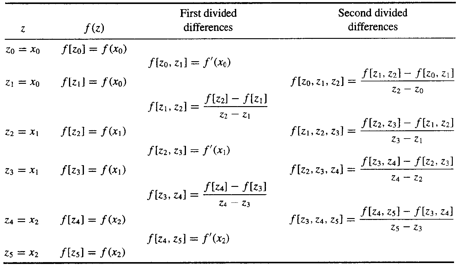
The theorem above gives a complete description of Hermit interpolation. But in pratice, to compute \(H_{2n + 1}(x)\) through the formula above is tedious. To make it compute easier, we introduce a method that is similar to Newton's interpolation.
Define the sequence \(\{z_k\}_{0}^{2n + 1}\) by
Based on the Theorem 3.4, we redefine that
Then Hermite polynomial can be represented by
Cubic Spline Interpolation
Motivation: For osculating polynomial approximation, we can let \(m_i\) be bigger to get high-degree polynomials. It can somehow be better but higher degree tends to causes a fluctuation or say overfitting.
An alternative approach is to divide the interval into subintervals and approximate them respectively, which is called piecewise-polynomial approximation. The most common piecewise-polynomial approximation uses cubic polynomials called cubic spline approximation.
Definition 3.4
Given a function \(f\) defined on \([a, b]\) and a set of nodes \(a = x_0 < x_1 < \cdots < x_n = b\), a cubic spline interpolant \(S\) for \(f\) is a function that satisfies the following conditions.
- \(S(x)\) is a cubic polynomial, denoted \(S_j(x)\), on the subinterval \([x_j, x_j + 1]\), for each \(j = 0, 1, \dots, n - 1\);
- \(S(x_j) = f(x_j)\) for each \(j = 0, 1, \dots, n\);
- \(S_{j + 1}(x_{j + 1}) = S_j(x_{j + 1})\) for each \(j = 0, 1, \dots, n - 2\);
- \(S'_{j + 1}(x_{j + 1}) = S'_j(x_{j + 1})\) for each \(j = 0, 1, \dots, n - 2\);
- \(S''_{j + 1}(x_{j + 1}) = S''_j(x_{j + 1})\) for each \(j = 0, 1, \dots, n - 2\);
- One of the following sets of boundary conditions:
- \(S''(x_0) = S''(x_n) = 0\) (free or natural boundary);
- \(S'(x_0) = f'(x_0)\) and \(S'(x_n) = f'(x_n)\) (clamped boundary).
The spline of natural boundary is called natural spline.
Theorem 3.6
The cubic spline interpolation of either natural boundary or clamped boundary is unique.
(Since the coefficient matrix \(A\) is strictly diagonally dominant.)
Suppose interpolation function in each subinterval is
From the conditions in the definition above, by some algebraic process, we can derive the solution with the following equations,
While \(c_j\) is given by solving the following linear system,
where
For natural boundary,
For clamped boundary,
For More Accuracy...
If \(f \in C[a, b]\) and \(\frac{\max h_i}{\min h_i} \le C < \infty\). Then \(S(x)\ \overset{\text{uniform}}{\longrightarrow}\ f(x)\) when \(\max h_i \rightarrow 0\).
That is the accuracy of approximation can be improved by adding more nodes without increasing the degree of the splines.
Curves
We've discussed the interpolation of functions above, but we may encounter the case to interpolate a curve.
Straightforward Technique
For given points \((x_0, y_0), (x_1, y_1), \dots, (x_n, y_n)\), we can construct two approximation functions with
The interpolation method can be Lagrange, Hermite and Cubic spline, whatever.
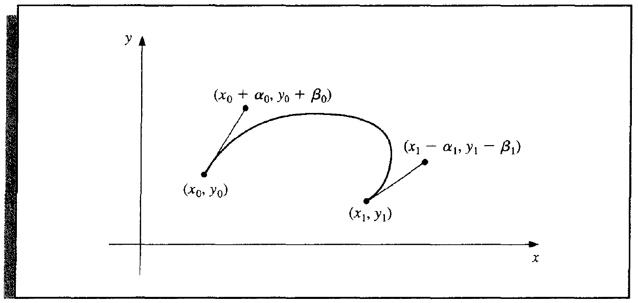
Bezier Curve
In nature, it's piecewise cubic Hermite polynomial, and the curve is called Bezier curve.
Similarly, suppose two function \(x(t)\) and \(y(t)\) at each interval. We have the following condtions.
The solution is
创建日期: 2022.11.10 01:04:43 CST