Lecture 5 Image Matching and Motion Estimation

Image Matching

Abstract

1. Dectection
2. Description
3. Matching
4. Learned based matching

1. Detection

We want uniqueness.

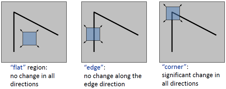
Corner Detection

Local measures of uniqueness

shifting the window in any direction causes a big change

distribution of gradients

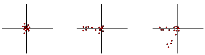
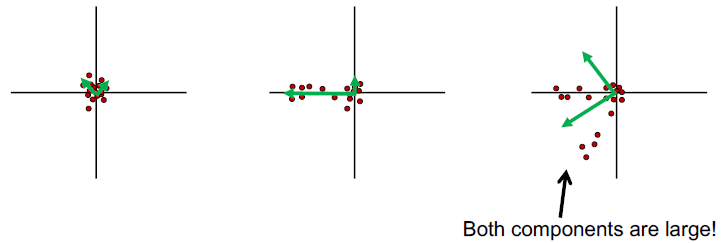
Principal Component Analysis (PCA) 主成分分析

To describe the distribution of gradients by two eigenvectors.

Method of Corner Detection

1. Compute the covariance matrix \(H\) at each point and compute its eigenvalues \(\lambda_1\), \(\lambda_2\).
2. Classification
   1. Flat - \(\lambda_1\) and \(lambda_2\) are both small.
   2. Edge - \(\lambda_1 \gg \lambda_2\) or \(\lambda_1 \ll \lambda_2\).
   3. Corner - \(\lambda_1\) and \(\lambda_2\) are both large.

Harris Corner Detector

However, computing eigenvalues are expensive. Instead, we use Harris corner detector to indicate it.

1. Compute derivatives at each pixel.
2. Compute covariance matrix \(H\) in a Gaussian window around each pixel.

3. Compute corner response function (Harris corner detector) \(f\), given by

   \[ f = \frac{\lambda_1\lambda_2}{\lambda_1 + \lambda_2} = \frac{\det(H)}{\text{tr}(H)}. \]

4. Threshold \(f\).

5. Find local maxima of response function.

Invariance Properties

• Invariant to translation, rotation and intensity shift.
• Not invariant to scaling and intensity scaling.
  • How to find the correct scale?
    • Try each scale and find the scale of maximum of \(f\).

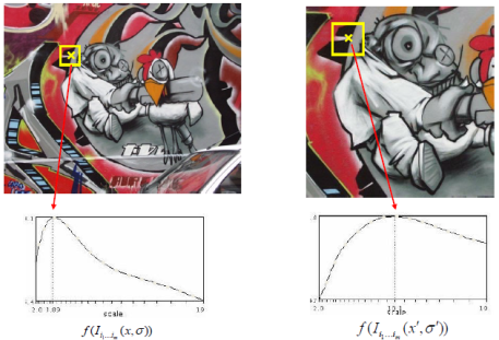
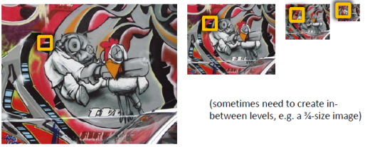
Implementation

image pyramid with a fixed window size.

Blob Detection

convolution!

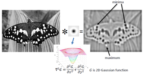
Laplacian of Gaussian (LoG) Filter

Example

\[ f = \begin{bmatrix} 0 & 1 & 0 \\ 1 & -4 & 1 \\ 0 & 1 & 0 \end{bmatrix}. \]

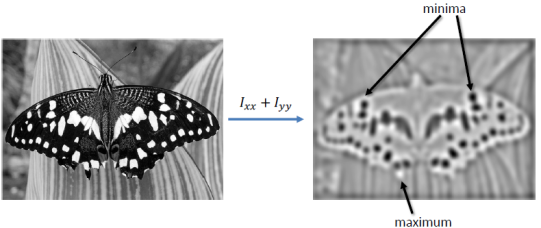
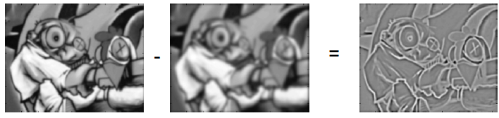
Laplacian is sensitive to noise. To solve this flaw, we often

1. Smooth image with a Gaussian filter
2. Compute Laplacian

\[ \nabla^2(f*g) = f*\nabla^2g, \text{ where $f$ is the Laplacian and $g$ is the Gaussian} \]

Scale Selection (the same problem as corner detection)

The same solution as corner detection - Try and find maximum.

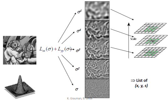
Implementation: Difference of Gaussian (DoG)

A way to acclerate computation, since LoG can be approximated by DoG.

\[ \nabla^2G_\sigma \approx G_{\sigma_1} - G_{\sigma_2} \]

2. Description

We mainly focus on the SIFT (Scale Invariant Feature Transform) descriptor.

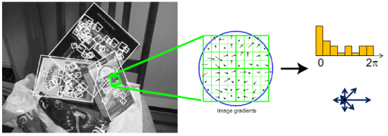
Orientation Normalization

1. Compute orientation histogram
2. Select dominant orientation
3. Normalize: rotate to fixed orientation

Properites of SIFT

• Extraordinaraily robust matching technique
  • handle changes in viewpoint
    • Theoretically invariant to scale and rotation
  • handle significant changes in illumination
  • Fast

Other dectectores and descriptors

• HOG
• SURF
• FAST
• ORB
• Fast Retina Key-point

3. Matching

Feature matching

• Define distance function to compare two descriptors.
• Test all to find the minimum distance.

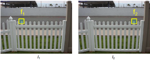
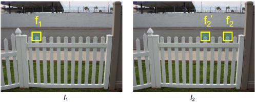
Problem: repeated elements

• To find that the problem happens: Ratio Test

• Ratio score = \(\frac{||f_1 - f_2||}{||f_1 - f_2'||}\)

• best match \(f_2\), second best match \(f'_2\).

• Another strategy: Mutual Nearest Neighbor
  • \(f_2\) is the nearest neighbour of \(f_1\) in \(I_2\).
  • \(f_1\) is the nearest neighbour of \(f_2\) in \(I_1\).

4. Learning based matching

Question

Motion Estimation

Problems

• Feature-tracking
• Optical flow

Method: Lucas-Kanade Method

Assumptions

1. Small motion
2. Brightness constancy
3. Spatial coherence

Brightness constancy

\[ \begin{aligned} I(x, y, t) &= I(x + u, y + v, t + 1) \\ I(x + u, y + v, t + 1) &\approx I(x, y, t) + I_x u + I_y v + I_t \\ I_x u + I_y v + I_t &\approx 0 \\ \nabla I \cdot [u, v]^T + I_t &= 0 \end{aligned} \]

Aperture Problem

Idea: To get more equations → Spatial coherence constraint

Assume the pixel's neighbors have the same motion \([u, v]\).

If we use an \(n\times n\) window,

\[ \begin{bmatrix} I_x(\textbf{p}_\textbf{1}) & I_y(\textbf{p}_\textbf{1}) \\ \vdots & \vdots\\ I_x(\textbf{p}_\textbf{1}) & I_y(\textbf{p}_{\textbf{n}^\textbf{2}}) \\ \end{bmatrix} \begin{bmatrix} u \\ v \end{bmatrix} = - \begin{bmatrix} I_t(\textbf{p}_\textbf{1}) \\ \vdots \\ I_t(\textbf{p}_{\textbf{n}^\textbf{2}}) \end{bmatrix} \Rightarrow Ad=b \]

More equations than variables. Thus we solve \(\min_d||Ad-b||^2\).

Solution is given by \((A^TA)d = A^Tb\), when solvable, which is \(A^TA\) should be invertible and well-conditioned (eigenvalues should not be too small, similarly with criteria for Harris corner detector).

Thus it's easier to estimate the motion of a corner, then edge, then low texture region (flat).

Small Motion Assumption

For taylor expansion, we want the motion as small as possbile. But probably not - at least larger than one pixel.

Solution

• Reduce the resolution

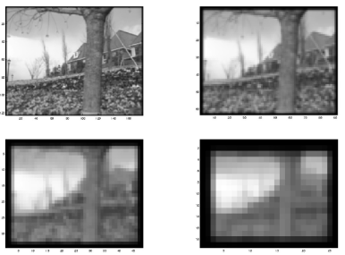
• Use the image pyramid

---

最后更新: 2023.11.21 17:00:13 CST
创建日期: 2022.11.10 01:04:43 CST