Graph¶

Definition

A Graph consists of vertices and edges. It can be represented by the mark $G(V, E)$, where

$G$ denotes the graph.
$V = V(G) = \{v_1, \dots, v_n\}$ denotes a finite nonempty set of vertices.
$E = E(G) = \{e_1, \dots, e_m\}$ denotes a finite set of edges.

When we discuss graph in this course FDS, we have the following restrictions

Self loop is illegal.

Multigraph is not considered.

Definition

Undirected graph (无向图): the edge from $v_i$ to $v_j$ is the same as that from $v_j$ to $v_i$, denoted by $(v_i, v_j) = (v_j, v_i)$.
Directed graph (digraph, 有向图): the edge from $v_i$ to $v_j$ is the different from that from $v_j$ to $v_i$, denoted by $<v_i, v_j> = <v_j, v_i>$.
Complete graph (完全图):
A graph that has the maximum number of edges.
- For a complete undirected graph with $n$ vertices, there are $\dfrac{n(n-1)}{2}$ edges.
- For a complete directed grach with $n$ vertices, there are $n(n-1)$ edges.
Adjacency (相邻):
- For an undirected graph, if there is an edge $(v_i, v_j)$, then $v_i$ and $v_j$ are adjacent and $(v_i, v_j)$ is incident* on $v_i$ and $v_j$.
- For a directed graph, if there is an edge $<v_i, v_j>$, then $v_i$ is adjacent to $v_j$, $v_j$ is adjacent from $v_i$ and $<v_i, v_j>$ is incident on $v_i$ and $v_j$.
Subgrach $G' \subset G$ (子图): $V(G') \subseteq V(G)$ and $E(G')\subseteq E(G)$.
Path from $v_p$ to $v_q$ (路径): $\{v_p, v_{i_1}, v_{i_2}, \cdots, v_{i_n}, v_q \}$ such that $(v_p,v_{i1}), (v_{i1}, v_{i2}), \dots, (v_{in}, v_q)$ or $<v_p,v_{i1}>, <v_{i1}, v_{i2}>, \dots, <v_{in}, v_q>$ are in $E(G)$.
- Length of a path (路径长度): number of edges on the path.
- Simple path (简单路径): $v_{i_1}, v_{i_2}, \dots, v_{i_n}$ are distinct.
- Cycle (环): a simple path with $v_p=v_q$.
Connection (连通性)
- For an undirected graph,
  - Connected vertices (连通点): there is a path from $v_i$ to $v_j$.
  - Connected graph (连通图): all pairs of distinct vertices are connected.
  - (Connected) Component (连通分量): the maximum connected subgraph.
- For a directed graph,
  - Strongly Connected (强连通): all pairs of distinct vertices are connected.
  - Weakly Connected (弱连通): the graph is connected without direction to the edges.
  - Strongly Connected Component (强连通分量): the maximum subgraph that is strongly connected.
Biconnection (双连通性) for an undirected graph $G$
- $v$ is an articulation point / cut point (割点) if $G'$, which is $G$ with vertex $v$ deleted has at least 2 connected components.
- $(v_i, v_j)$ is an bridge / cut edge (桥 / 割边) if $G'$, which is $G$ with edge $(v_i, v_j)$ deleted has at least 2 connected components.
- $G$ is a biconnected graph (双连通图) if $G$ is connected and has no articulation points.
- A biconnected component (双连通分量) is a maximal biconnected subgraph.
A Tree: a graph that is connected and acyclic.
A DAG (有向无环图): a directed acyclic graph.
Degree (度): number of edges incident to $v$.
- For a directed $G$, we have indegree (入度) as the edges to $v$ and outdegree (出度) as the edges from $v$
- If there is a graph $G$ with $n$ vertices and $e$ edges, then
  
  \[ e=\frac12\sum\limits_{i=0}^{n-1}degree(v_i). \]

Representation¶

NOTE that all vertices of a graph with $n$ vertices are numbered from $0$ to $n - 1$.

Weighted Edges In some cases, we want each edge has a weight $w$. In particular, when weight isn't considered, it's same to treat all weight be $1$.

Data Type

typedef struct {
    int u; // start vector
    int v; // end vector
    int w; // weight
} Edge;

Adjacency Matrix 邻接矩阵¶

Use a matrix to represent the edges of a graph.

\[ \text{AdjacencyMatrix}[i][j] = \left\{ \begin{aligned} & 1 \text{ or } \text{weight}, && \text{if } (v_i,v_j) \text{ or } <v_i,v_j>\ \in E(G), \\ & 0, && \text{otherwise}. \end{aligned} \right. \]

Data Type

typedef struct {
    int n; // number of vertices
    int m; // number of edges
    int **adjMat;
} Graph;

Adjacency Matrix of Digraph

Graph *CreateGraph(const int n) {
    Graph *G = (Graph *)malloc(sizeof(Graph));
    G->n = n;
    G->m = 0;
    G->adjMat = (int **)malloc(G->n * sizeof(int *));
    G->adjMat[0] = (int *)malloc(G->n * G->n * sizeof(int));
    for (int i = 1; i < G->n; i ++) {
        G->adjMat[i] = G->adjMat[0] + i * G->n;
    }
    return G;
}

void AddEdge(Graph *G, const Edge e) {
    G->m ++;
    G->adjMat[e.u][e.v] = e.w;
}

void FreeGraph(Graph *G) {
    free(G->adjMat[0]);
    free(G->adjMat);
    free(G);
}

Pros

Easy for implementation.
Fast to reach.

Cons

Space complexity $O(n^2)$, which is a waste when representing a sparse graph.

Adjacency Lists 邻接链表¶

Replace each row of the adjacency matrix by a linked list. The order of vertices in each list doesn't matter.

Data Type

typedef struct _node {
    int to;
    int w;
    struct _node *next;
} Node;

typedef struct {
    int size;
    Node *head;
} List;

typedef struct {
    int n;
    int m;
    List **adjList;
} Graph;

Adjacency Lists of Digraph

void Insert(List *list, const int to, const int w) {
    Node *p = (Node *)malloc(sizeof(Node));
    p->to = to;
    p->w = w;
    p->next = list->head->next;
    list->head->next = p;
}

Graph *CreateGraph(const int n) {
    Graph *G = (Graph *)malloc(sizeof(Graph));
    G->n = n;
    G->m = 0;
    G->adjList = (List **)malloc(G->n * sizeof(List *));
    for (int i = 0; i < G->n; i ++) {
        G->adjList[i] = (List *)malloc(sizeof(List));
        G->adjList[i]->size = 0;
        G->adjList[i]->head = (Node *)malloc(sizeof(Node));
        G->adjList[i]->head->next = NULL;
    }
    return G;
}

void AddEdge(Graph *G, const Edge e) {
    G->m ++;
    Insert(G->adjList[e.u], e.v, e.w);
}

void FreeGraph(Graph *G) {
    for (int i = 0; i < G->n; i ++) {
        for (Node *p = G->adjList[i]->head, *temp = NULL; p != NULL;) {
            temp = p;
            p = p->next;
            free(temp);
        }
        free(G->adjList[i]);
    }
    free(G->adjList);
    free(G);
}

Pros

Save space.

Cons

Complicated for implementation.

Adjacency Multilists 链式前向星¶

Use the edges as nodes of multilists, and represent it by something similar with a static list.

Data Type

typedef struct {
    int to;
    int w;
    int next;
} EdgeNode;

typedef struct {
    int n;
    int m;
    EdgeNode *edge;
    int *head;
} Graph;

Adjacency Multilists

Graph *CreateGraph(const int n, const int m) { // (1)!
    Graph *G = (Graph *)malloc(sizeof(Graph));
    G->n = n;
    G->m = m;
    G->edge = (EdgeNode *)malloc(G->m * sizeof(EdgeNode));
    G->head = (int *)malloc(G->n * sizeof(int));
    memset(G->edge, 0, G->m * sizeof(EdgeNode));
    for (int i = 0; i < G->n; ++ i) {
        G->head[i] = -1;
    }
    G->m = 0;
    return G;
}

void AddEdge(Graph *G, const Edge e) {
    G->edge[G->m].to = e.v;
    G->edge[G->m].w = e.w;
    G->edge[G->m].next = G->head[e.u];
    G->head[e.u] = G->m;
    G->m ++;
}

void FreeGraph(Graph *G) {
    free(G->edge);
    free(G->head);
    free(G);
}

Note that for undirected graph, m should be pass by 2 * m.

Example: How Adjacency Multilists Build

for the left given graph, the corresponding adjancency multilists is the right one

Topological Sort¶

Definition

AOV Network (Activity On Vertex Network) is a digraph $G$ in which $V(G)$ represents activities and $E(G)$ represents precedence relations between activities (vertices).

$i$ is a predecessor of $j$ if there is a path from $i$ to $j$,
$i$ is an immediate predecessor of j if $<i,j> \in E(G)$, and $j$ is called a successor(immediate sucessor) of $i$. If we can finish all activities in AOV Network in any order without finishing one before its predecessor finished, the AOV Network is feasible, else it is unfeasible

Patial order is a precedence relation which is both transitive and irrelative.

Proposition

A project is feasible if it's irreflexive. Otherwise $i$ is a predecessor of $i$, which means that $i$ must be done before $i$ starts.

Feasible AOV network must be a DAG.

Definition | Topological Order

A topological order is a linear ordering of the vertices of a graph such that, for any two vertices $i$ and $j$, if $i$ is a predecessor of $j$ in the network then $i$ precedes $j$ in the linear ordering.

Topological Sort

void FindIndegree(const Graph *G, int indegree[]) {
    memset(indegree, 0, G->n * sizeof(int));
    for (int i = 0; i < G->n; i ++) {
        for (int j = G->head[i]; j != -1; j = G->edge[j].next) {
            indegree[G->edge[j].to] ++;
        }
    }
}

void TopologicalSort(const Graph *G, int topNum[]) { // (1)!
    Queue *queue = CreateQueue(G->m);
    int indegree[G->n];
    FindIndegree(G, indegree);
    for (int i = 0; i < G->n; i ++) {
        if (indegree[i] == 0) {
            Enqueue(queue, i);
        }
    }
    int cnt = 0;
    while (!IsEmptyQueue(queue)) {
        int now = Dequeue(queue);
        topNum[cnt ++] = now;
        for (int idx = G->head[now]; idx != -1; idx = G->edge[idx].next) { //(2)!
            int to = G->edge[idx].to;
            indegree[to] --;
            if (indegree[to] == 0) {
                Enqueue(queue, to);
            }
        }
    }
    if (cnt != G->n) {
        puts("Graph has a cycle");
    }
}

1.topNum[] stores the result of topological sort. 2. The graph is represented by adjacent multilists. Other representations are also available.

Complexity

Suppose $E$ is the number of edges and $V$ is the number of vertices, then

Time complexity $O(E + V)$.
Space complexity $O(V)$.

Note

Topological sort can be used to detect whether the graph has a cycle, and it can also be used to detect whether the graph is a chain.
Topological sort is not unique.

Shortest Paths¶

Definition

Given a digraph $G=(V,E)$, and a cost function $c(e)$ for $e\in E(G)$, the length of a path $P$ (also called weighted path length) from source to destination is $\sum\limits_{e_i\subset P}\ w(e_i)$.

The result of the following algorithms are stored in the following data type.

Data Type

typedef struct {
    int dist;
    bool vis;
    int prev;
} Path;

dist is the distance from source to v_i.
vis is set to false if v_i is visited or true if not.
prev record the previous vertex along the path. We can trace back until prev = -1 to obtain the path from source to v_i.

Trace Back of Vertex v

int now = v;
while (now != -1) {
    printf("%d ", now);
    now = path[now].prev;
}

Unweight Shortest Paths¶

It is implemented by a breadth-first search (BFS) algorithm, which used to find how many vertices from source to destination.

Unweighted Shortest Paths

#define INF 0x3f3f3f

void BFS(const Graph *G, const int source, Path path[]) {
    for (int i = 0; i < G->n; i ++) {
        path[i].dist = INF;
        path[i].vis = false;
        path[i].prev = -1;
    }
    path[source].dist = 0;

    Queue *queue = CreateQueue(G->n);
    Enqueue(queue, source);
    while (!IsEmptyQueue(queue)) {
        int now = Dequeue(queue);
        path[now].vis = true;
        for (int idx = G->head[now]; idx != -1; idx = G->edge[idx].next) { //(1)!
            int to = G->edge[idx].to;
            if (!path[to].vis) {
                path[to].dist = path[now].dist + 1;
                path[to].prev = now;
                Enqueue(queue, to);
            }
        }
    }
    FreeQueue(queue);

    return path;
}

The graph is represented by adjacent multilists. Other representations are also available.

Reason to Choose INF to be 0x3f3f3f

We can use memset(a, 0x3f, n * sizeof(int)) to initialze.
Add two infinities will still result in an infinity.

Complexity

Time complexity $O(E + V)$.
Space comlexity $O(E)$.

Weighted Shortest Paths¶

Floyd¶

Remains

Dijkstra¶

Description of Dijkstra

Let $S = \{ s \text{ and } v_i \text{'s whose shortest paths have been found}\}$. For any $u \notin S$, define

\[ \text{distance}[u] = \text{minimal length of path} \{ s \rightarrow (v_i\in S)\rightarrow u \}. \]

If the paths are generated in non-decreasing order, then

The shortest path must go through ONLY $v_i \in S$
(Greedy Method) $u$ is chosen so that $\text{distance}[u] = \min\{w \notin S | \text{distance}[w]\}$ (If $u$ is not unique, then we can choose any of them).
If $\text{distance} [u_1] < \text{distance} [u_2]$ and we add $u_1$ into $S$, then distance$[u_2]$ may change. If so, a shorter path from $s$ to $u_2$ must go through $u_1$ and

\[ \text{distance}'[u_2] = \text{distance} [u_1] + \text{length}(<u_1,u_2>). \]

Note

For finding $u$, we can maintain a priority queue, which can decrease time complexity of finding $u$ from $O(V)$ to $O(\log V)$.

Dijkstra's Algorithm

SimpleImproved by Priority Queue

void Dijkstra(const Graph *G, const int source, Path path[]) {
    for (int i = 0; i < G->n; i ++) {
        path[i].dist = INF;
        path[i].vis = false;
        path[i].prev = -1;
    }
    path[source].dist = 0;

    int now = source;
    while (!path[now].vis) {
        path[now].vis = true;

        for (int idx = G->head[now]; idx != -1; idx = G->edge[idx].next) {
            int to = G->edge[idx].to;
            int cost = G->edge[idx].dis;
            if (path[to].dist > path[now].dist + cost) {
                path[to].dist = path[now].dist + cost;
                path[to].prev = now;
            }
        }

        int distMin = INF;
        for (int i = 0; i < G->n; i ++) {
            if (!path[i].vis && path[i].dist < distMin) {
                distMin = path[i].dist;
                now = i;
            }
        }
    }
}

typedef struct {
    int num;
    int dis;
} Node;

#define MinData -1
typedef Node ElementType;
typedef struct {
    ElementType *element;
    int capacity;
    int size;
} PriorityQueue;

...

void Dijkstra(const Graph *G, const int source, Path path[]) {
    for (int i = 0; i < G->n; i ++) {
        path[i].dist = INF;
        path[i].vis = false;
        path[i].prev = -1;
    }
    path[source].dist = 0;

    PriorityQueue *Q = Initialize(G->m);
    Insert(Q, (Node){source, 0});

    while (!IsEmptyQueue(Q)) {
        Node cur = DeleteMin(Q);
        int now = cur.num;

        if (path[now].vis) {
            continue;
        }
        path[now].vis = true;

        for (int idx = G->head[now]; idx != -1; idx = G->edge[idx].next) {
            int to = G->edge[idx].to;
            int cost = G->edge[idx].dis;
            if (path[to].dist > path[now].dist + cost) {
                path[to].dist = path[now].dist + cost;
                                path[to].prev = now;
                if (!path[to].vis) {
                    Insert(Q, (Node){to, path[to].dist});
                }
            }
        }
    }
}

Complexity

Time complexity
- Simple $O(E + V^2)$.
- Improved $O((E + V) \log V)$.
Space comlexity
- Simple $O(1)$.
- Improved $O(E)$.

Warning

By allowing the used vertices being pushed into the set $S$ again, we can get a algorithm that deals with negative edges well with time complexity $T = O(E \cdot V)$. However, if the graph has a negative-weight cycle, it will cause infinite loop.

SPFA¶

Remains

Acyclic Graph¶

If the graph is acyclic, vertices may be selected in topological order since when a vertex is selected, its distance can no longer be lowered without any incoming edges from unknown nodes

$T=O(|E|+|V|)$ and no priority queue is needed

All-Pairs Shortest Path Problem¶

Use single-source algorithm for $V$ times with $T=O(V^3)$ - works fast on sparse graph.

Remains

Another $O(|V|^3)$ algorithm in book's Chapter 10 - works faster on dense graphs

Network Flow Problems¶

Definition | Network

A network is a digraph $G(V, E)$. Each edge $(u, v) \in E(G)$ has a weight $c(u, v)$ called capacity. In particular, $\forall\ (u, v) \notin E(G)$, $c(u, v) = 0$. Moreover, there are two special points, source (源点) $s$ and sink (汇点) $t$ ($s \ne t$).

Definition | Flow

If $f(u, v)$ is a function that satisfies

Capacity Restriction: $f(u, v) \le c(u, v)$.
Skew Symmetry: $f(u, v) = -f(v, u)$.
Conservation of Flow: sum of outflows of source equals to sum of inflows of sink.

\[ \forall\ x \in V - {s, t},\ \ \sum\limits_{(u, x) \in E} f(u, x) = \sum\limits_{(x, v) \in E} f(x, v). \]

Maximum Flow¶

Maximum flow probelm want to determine the maximum amount of flow that can pass from source $s$ to sink $t$.

We introduce Ford-Fulkerson Augmenting Path Algorithm here.

Definition

Residual capacity $c_f(u, v)$ is defined by the subtraction between the capacity of the edge and the flow, namely $c_f(u, v) = c(u, v) - f(u, v)$.

A residual network $G_f$ is the graph consists of all vertices of $G$ and all edges that residual capacity is larger than $0$, namely $G_f = (V_f = V, E_f = \{(u, v) \in E | c_f(u, v) > 0\})$.

An augmenting Path (增广路) is a path from $s$ to $t$, with each edge using the minimum residual capacity of edges in the path.

Proposition

If the edge capabilities are rational numbers, this algorithm always terminate with a maximum flow.

Note

The algorithm works for $G$ with cycles as well.

Basic Idea

Find an augmenting path from $s$ to $t$.
Augment it by
- subtracting minimum residual capacity along the augmenting path.
- adding minimum residual capacity along the inverse augmenting path.

Example

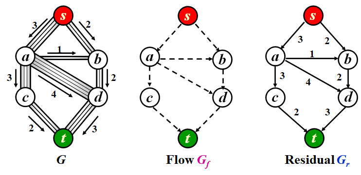
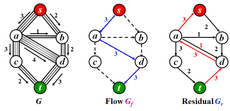
Description

$G_r$ is initialized to be the same as $G$ to represent the selected flows. $G_f$ is just a assistant graph of selected augmenting path.
First, we find the blue augmenting path from $s$ to $t$ in $G_f$. The minimum residual capacity along tha path is $3$. Then we subtract $3$ along the path, and add $3$ along the inverse path.
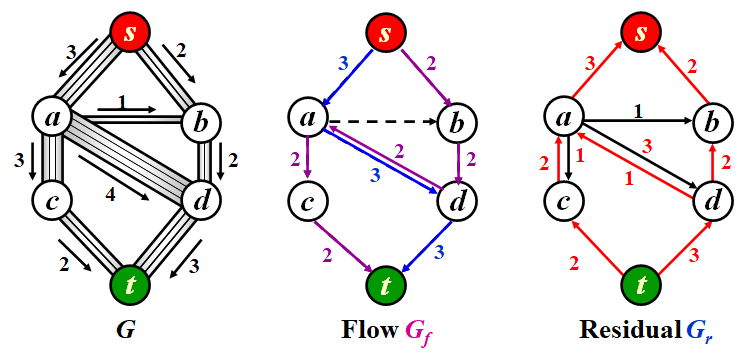
Second, we find the purple augmenting path from $s$ to $t$ in $G_f$. The minimum residual capacity along tha path is $2$. Then we subtract $2$ along the path, and add $2$ along the inverse path.
Since there is no outflows of $s$ in $G_f$, we can't find any augementing path any more. Thus it's the result case.

Ford-Fulkerson Augmenting Path Algorithm

DFSEdomnds-Karp / EK (BFS)

int dfs(const int now, const int prevCapacity, Graph *G, bool vis[], const int s, const int t) {
    if (now == t) {
        return prevCapacity;
    }

    vis[now] = true;
    for (int idx = G->head[now]; idx; idx = G->edge[idx].next) {
        int to = G->edge[idx].to;
        int capacity = G->edge[idx].capacity;

        if (capacity == 0 || vis[to] == true) {
            continue;
        }

        int cost = dfs(to, min(capacity, prevCapacity), vis, s, t, G);
        if (cost != -1) {
            G->edge[idx].capacity -= cost;
            G->edge[idx ^ 1].capacity += cost;
            return cost;
        }
    }
    return -1;
}

int FF(Graph *G, const int s, const int t) {
    int ret = 0, cost;
    bool vis[G->n];

    memset(vis, false, G->n * sizeof(bool));
    while ((cost = dfs(s, 0x3f3f3f, vis, s, t, G)) != -1) {
        memset(vis, false, G->n * sizeof(bool));
        ret += cost;
    }
    return ret;
}

Remains

Complexity

Suppose all capacity is integers, we have serval methods to find an augmenting path.

Choose the augmenting path found by an unweighted shortest path algorithm.
- Time complexity
  
  \[ \begin{aligned} T &= T_{\text{augmentation}} \cdot T_{\text{find a path}} \\ &= O(f) \cdot O(E) \\ &= O(f\cdot E),\ \ \text{ where $f$ is the maximum flow.} \end{aligned} \]
Choose the augmenting path that allows the largest increase in flow found by Dijkstra's algorithm.
- Time complextiy
  
  \[ \begin{aligned} T &= T_{\text{augmentation}} \cdot T_{\text{find a path}} \\ &= O(E\log cap_{\text{max}}) \cdot O(E\log V) \\ &= O(E^2\log V),\ \ \text{if $cap_{\text{max}} = \max\{c(u, v)\}$ is small}. \end{aligned} \]
Choose the augmenting path that has the least number of edges found by unweighted shortest path algorithm.
- Time complexity
  
  \[ \begin{aligned} T &= T_{augmentation} \cdot T_{find a path} \\ &= O(E) \cdot O(E \cdot V) \\ &= O(E^2V). \end{aligned} \]

Proposition

If every $v\notin {s,t}$ has either a single incoming edge of capacity $1$ oe a single outgoing edge of capacity $1$, then time bound is reduced to $O(E V^{1/2})$.

Min Cost Flow¶

The min-cost flow problem want to find among all maximum flows, the one flow of minimum cost provided that each edge has a cost per unit of flow.

Remains

Minimum Spanning Tree (MST)¶

Definition

A spanning tree of a graph $G$ is a tree which consists of $V(G)$ and a subset of $E(G)$.

A minimum spanning tree (MST) is a spanning tree that the total cost of its edges is minimized.

Note

MST is a tree since it is acyclic, and thus the number of edges is $V-1$. It is spanning because it covers every vertex.
A minimum spanning tree exists iff $G$ is connected (in most case it's undirected).
Adding a non-tree edge to a spanning tree, it becomes a cycle.

Kruskal's Algorithm¶

It maintains a forest and is implemented by Disjoint Set. Basic idea is adding one edge at one time in an non-decreasing order and it's a Greedy Method.

Results of Kruskal are stored in the following data type.

Data Type

typedef struct {
    int n;          // number of vertices in MST.
    int *vertex;    // vertices in MST.
    int edgeSum;    // sum of the weight of edges in MST.
} Point;

Kruskal's Algorithm

int cmp(const void *a, const void *b) {
    return ((Edge *)a)->w - ((Edge *)b)->w;
}

int Find(int *S, const int a) {
    if (S[a] < 0) {
            return a;
    }
    return S[a] = Find(S, S[a]);
}

void Union(int *S, const int root_a, const int root_b) {
    if (root_a < root_b) {
            S[root_a] += S[root_b];
            S[root_b] = root_a;
    } else {
            S[root_b] += S[root_a];
            S[root_a] = root_b;
    }
}

void Kruskal(Graph *G, Point *point) {
    Edge edge[G->m];
    for (int i = 0, cnt = 0; i < G->n; i ++) {
            for (int idx = G->head[i]; idx != -1; idx = G->edge[idx].next) {
                    edge[cnt ++] = (Edge){i, G->edge[idx].to, G->edge[idx].w};
            }
    }
    qsort(edge, G->m, sizeof(Edge), cmp);

    int *S = (int *)malloc(G->n * sizeof(int));
    for (int i = 0; i < G->n; ++ i) {
            S[i] = -1;
    }

    int cnt = 0, vertex[G->n], sum = 0;
    for (int i = 0; i < G->m; ++ i) {
        int root_a = Find(S, edge[i].u);
        int root_b = Find(S, edge[i].v);

        if (root_a == root_b) {
            continue;
        }

        Union(S, root_a, root_b);
        vertex[cnt ++] = i;
                sum += edge[i].w;
    }

    point->n = cnt;
    point->vertex = (int *)malloc(point->n * sizeof(int));
    memcpy(point->vertex, vertex, cnt * sizeof(int));
    point->edgeSum = sum;

    free(S);
}

Complexity

Time complexity $O(E\log E)$ (sorting algorithm of $O(E \log E)$, and union-find of $O(E \alpha(V))$ or $O(E \log V)$).
Space complexity $O(V)$.

Prim's Algorithm¶

Basic idea is adding one vertex at one time to grow a tree, very similar to Dijkstra's algorithm. $T=O(|E|\log|V|)$.

Prim's Algorithm

SimpleImprove by Priority Queue

void Prim(Graph *G, Point *point) {
    int dist[G->n], prev[G->n];
    bool vis[G->n];

    memset(vis, false, sizeof(vis));
    memset(dist, 0x3f, sizeof(dist));

    int cnt = 0, vertex[G->n], sum = 0;

    int now = 0;
    dist[now] = 0;
    for (int r = 0; r < G->n; r ++) {
        vis[now] = true;
        if (r != 0) {
            sum += G->adjMat[prev[now]][now];
        }
        vertex[cnt ++] = now;

        for (int i = 0; i < G->n; i ++) {
            if (!vis[i] && G->adjMat[now][i] < dist[i]) {
                    dist[i] = G->adjMat[now][i];
                    prev[i] = now;
            }
        }

        int minDist = 0x3f3f3f;
        for (int i = 0; i < G->n; i ++) {
            if (!vis[i] && dist[i] < minDist) {
                    now = i;
                    minDist = dist[i];
            }
        }
    }

    point->n = cnt;
    point->vertex = (int *)malloc(cnt * sizeof(int));
    memcpy(point->vertex, vertex, cnt * sizeof(int));
    point->edgeSum = sum;
}

Complexity

Time complexity
- Simple $O(E + V^2)$.
- Improved $O((E + V) \log V)$.
Space complexity $O(V)$.

Depth-First Search¶

DFS can be regarded as a generalization of preorder traversal. DFS of a graph can generate a spanning tree, called DFS spanning tree.

void DFS(Vertex V) {   
    vis[V] = true;  /* mark this vertex to avoid cycles */
    for (each W adjacent to V) {
        if (!vis[W]) {
            DFS(W);
        }
    }
}

Complexity

Time complexity $O(E + V)$.
Space complexity $O(1)$.

Tarjan Algorithm¶

Tarjan algorithm is used to find strongly connected components as well as cut point.

Define $\text{Low}(u)$ by

\[ \begin{aligned} \text{Low}(u) = \min\{ & \text{Index}(u), \\ & \min\{\text{Low}(w) | w \text{ is a child of } u\}, \\ & \min\{\text{Index}(w) | (u, w) \text{ is a back edge}\}. \end{aligned} \]

Strongly Connected Components (SCC)¶

For finding SCC, tarjan algorithm maintains a DFS spanning tree and a stack.

Tarjan Algorithm for Strongly Connected Components

void Tarjan(const int now, const Graph *G, int dfn[], int low[], Stack *stack, bool inStack[]) {
    static int idx = 0;

    dfn[now] = low[now] = ++ idx;
    inStack[now] = true;
    Push(stack, now);

    for (int i = G->head[now]; i != -1; i = G->edge[i].next) {
        int to = G->edge[i].to;
        if (dfn[to] == 0) {
            Tarjan(to, G, dfn, low, stack, inStack);
            low[now] = min(low[now], low[to]);
        } else {
            if (inStack[to]) {
                low[now] = min(low[now], dfn[to]);
            }
        }
    }

    if (dfn[now] == low[now]) {
        int temp;
        do {
            temp = Pop(stack);
            inStack[temp] = false;
            printf("%d", temp)
        } while (now != temp);
        putchar('\n');
    }
}

void FindStronglyConnectedComponents(const Graph *G) {
    int dfn[G->n], low[G->n];
    memset(dfn, 0, G->n * sizeof(int));
    memset(low, 0, G->n * sizeof(int));

    Stack *stack = CreateStack(G->n);
    bool inStack[G->n];
    memset(inStack, false, G->n * sizeof(bool));

    for (int i = 0; i < G->n; i ++) {
        if (dfn[i] == 0) {
            Tarjan(i, G, dfn, low, stack, inStack);
        }
    }
}

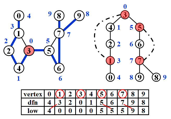
Cut Point¶

$u$ is an articulation point if

$u$ is the root and has at least 2 children.
$u$ is not the root, and has at least 1 child such that $\text{Low}(child) \ge \text{Index}(u)$.

Example

Suppose DFS spanning tree starts from vertex $3$. Blue numbers are indices of searching order stored in dfn[] and red points are the cut points.

Tarjan Algorithm for Articulation Point / Cut Point

void Tarjan(const int now, const Graph* G, const int root, int dfn[], int low[], bool isCutPoint[]) {
    static int idx = 0;

    int child = 0;
    dfn[now] = low[now] = ++ idx;

    for (int i = G->head[now]; i != -1; i = G->edge[i].next) {
        int to = G->edge[i].to;
        if (dfn[to] == 0) {
            child ++;
            Tarjan(to, G, root, dfn, low, isCutPoint);
            low[now] = min(low[now], low[to]);

            if (dfn[now] <= low[to] && now != root) {
                isCutPoint[now] = true;
            }
        }
        else {
            low[now] = min(low[now], dfn[to]);
        }
    }

    if (child > 1 && now == root) {
        isCutPoint[now] = true;
    }
}

void FindCutPoint(const Graph *G, bool isCutPoint[]) {
    int dfn[G->n], low[G->n];

    memset(dfn, 0, G->n * sizeof(int));
    memset(low, 0, G->n * sizeof(int));

    memset(isCutPoint, false, G->n * sizeof(bool));
    for (int i = 0; i < G->n; i ++) {
        if (dfn[i] == 0) {
            Tarjan(i, G, i, dfn, low, isCutPoint);
        }
    }
}

Euler Paths and Circuits¶

Definition

Euler tour / Path is a path go through all edges.

Euler circuit is a path go through all edges and finish at the starting point.

Theorem

An Euler circuit is possible only if the graph is connected and each vertex has an even degree

An Euler tour is possible if there are exactly two vertices having odd degree. One must start at one of the odd-degree vertices.

Note

The path should be maintained as a linked list
For each adjacency list, maintain a pointer to the last edge scanned
$T=O(|E|+|V|)$

Hamilton Paths and Circuits¶

Definition

Hamilton tour / Path is a path go through all vertices.

Hamilton circuit is a path go through all vertices and finish at the starting point.

最后更新: 2023.11.21 17:00:13 CST
创建日期: 2022.11.10 01:04:43 CST